Discrete_specific_techniques_dl

1. Bag of words (BOW)

BOW is a method to extract features from text documents, which is usually used in NLP, Information retrieve (IR) from documents and document classification. In general, BOW summarizes words in documents into a vocabulary (like dict type in python) that collects all the words in the documents along with word counts but disregarding the order they appear.

For examples, two sentences:

Lei Li would like to have a lunch before he goes to watch a movie.

James enjoyed the movie of Star War and would like to watch it again.

BOW will collect all the words together to form a vocabulary like:

{"Lei":1, "Li":1, "would":2, "like":2, "to":3, "have":1, "a":2, "lunch":1, "before":1, "he":1, "goes":1, "watch":2, "movie":2, "James":1, "enjoyed":1, "the":1, "of":1, "Star":1, "War":1, "and":1, "it":1, "again":1 }

The length of vector represents each sentence is equal to the word number, which is 22 in our case. Then first sentence is presented in vector (in the order of vocabulary) as: {1,1,1,1,2,1,2,1,1,1,1,1,1,0,0,0,0,0,0,0,0,0}, and the second sentence is presented in vector as: {0,0,1,1,1,0,0,0,0,0,0,1,1,1,1,1,1,1,1,1,1,1}.

Reference

https://www.freecodecamp.org/news/an-introduction-to-bag-of-words-and-how-to-code-it-in-python-for-nlp-282e87a9da04/

2. Principal Component Analysis (PCA)

To better understand the mathematic theory behind PCA, please refer to this Blog (Chinese only).

1. mean: $\mu_i = \frac{1}{n} \Sigma_{i=1}^n{x_i}$
2. variance: $\sigma^2 = \frac{1}{n} \Sigma_{i=1}^n{(x_i - \mu_i)^2}$
3. standard deviation: $\sigma^2 = \frac{1}{n-1} \Sigma_{i=1}^n{(x_i - \mu_i)^2}$
4. covariance: $cov(x,y) = \frac{1}{n-1} \Sigma_{i=1}^n{(x_i-\mu_x)*(y_i -\mu_y)}$

Let’s denote the input data $X$ is a $N \times M$ matrix where $N$ is the dimension of each input sample and $M$ is the number of input samples. Usually, the PCA aims to reduce the dimension $N$ to $R$ by a linear transformation matrix $P$ of $X$, which can be written as $Y=PX$. The dimension reduction actually changes the basis vector set of $X$ to the row vectors in $P$, and we hope the new basis vector set is independent from each other and the projected points in one basis vector is as far as possible from each other. In other words, we hope the variance in one basis vector is as large as possible and the covariance between each two basis vector is as small as possible. To this end, we compute the covariance matrix $B$ of $Y$, and we find the elements at diagonal are variances and other elements are covariance of new each basis vectors (in fact, the covariance matrix B is a symmetry matrix), thus we then seek $P$ to make the covariance matrix $B$ diagonalization, whcih means the elements are as large as possible at diagonal and elsewhere is zero.

$$B = \frac{1}{m} YY^T = \frac{1}{m} (PX)(PX)^T = P (\frac{1}{m}XX^T) P^T = P A P^T$$ where A denotes the covariance matrix of input data $X$. Equation above indicates that the $P$ diagonalize A is what we seek. In linear algebra, $P$ is actually made of eigenvectors of $A$ and elements at diagnoal are corresponding eigenvalues, which is called eigen decomposition. Based on this, we only need to compute the eigenvectors and their eigenvalues of $A$ and sort the eigenvectors into a matrix $C$ by ordering from larger corresponding eigenvalues to smaller ones. If we want to reduce the dimension from $N$ to $R$ ($R<N$), then we choose the top $R$ rows of $C$ to form $P$, and perform $PX$ to get the final result $Y$.

As we can see, PCA needs to compute the mean, variance and covariance to form the covariance matrix of original input data, and compute eigenvectors and their corresponding eigenvalues, which indicates this could be quite slow when input dimension $N$ is large.

Reference

https://blog.csdn.net/u010376788/article/details/46957957

3. Cross Entropy

3.1 Amount of information that an event gives

In general, the amount of information should be greater when an event with low probability happens. For example, event A: China won the table-tennis world champion; event B: Eygpt won the table-tennis world champion. Obviously, event B will give people more information if it happens. The reason behind this is that event A has great probability to happen while event B is rather rare, so people will get more information if event B happens.

The amount of information that an event gives is denoted as following equation:

$$f(x) = -log(p(x))$$ where $p(x)$ denotes the probability that event $x$ happens.

3.2 Entropy

For a given event $X$, there may be several possible situations/results, and each situation/result has its own probability, then the amount of information that this event gives is denoted as: $$f(X)= -\Sigma_{i=1}^{n}p(x_i)log(p(x_i))$$
where $n$ denotes the number of situations/results and $p(x_i)$ is the probability of situation/result $x_i$ happens.

3.3 Kullback-Leibler (KL) divergence

The KL divergence aims to describe the difference between two probability distributions. For instance, for a given event $X$ consisting of a series events ${x_1,x_2,…,x_n}$, if there are two probability distributions of possible situations/results: $P={p(x_1),p(x_2),…,p(x_n)}$ and $Q={q(x_1),q(x_2),…,q(x_n)}$, then the KL divergence distance between $P$ and $Q$ is formulated as:

$$D_{KL}(P||Q) = \Sigma_{i=1}^n p(x_i)log(\frac{p(x_i)}{q(x_i)})$$ further, $$D_{KL}(P||Q) = \Sigma_{i=1}^n p(x_i)log(p(x_i)) - \Sigma_{i=1}^n p(x_i)log(q(x_i))$$ where $Q$ is closer to $P$ when $D_{KL}(P||Q)$ is smaller.

3.4 Cross Entropy

In machine learning or deep learning, let $y={p(x_1),p(x_2),…,p(x_n)}$ denote the groundturth probability distribution, and $\widetilde{y}={q(x_1),q(x_2),…,q(x_n)}$ present the predicted probability distribution, then KL divergence is just a good way to compute the distance between predicted distribution and groudtruth. Thus, the loss could be just formulated as: $$Loss(y,\widetilde{y}) = \Sigma_{i=1}^n p(x_i)log(p(x_i)) - \Sigma_{i=1}^n p(x_i)log(q(x_i))$$ where the first term $\Sigma_{i=1}^n p(x_i)log(p(x_i))$ is a constant, then the $Loss(y,\widetilde{y})$ is only related to the second term $- \Sigma_{i=1}^n p(x_i)log(q(x_i))$ which is called **Cross Entropy** as a training loss.

Reference

https://blog.csdn.net/tsyccnh/article/details/79163834

4. Conv 1x1

Conv 1x1 in Google Inception is quite useful when the filter dimension of input featues needs to be increased or decreased meanwhile keeping the spaital dimension, and reduces the convolution computation. For example, the input feautre dimension is $(B, C, H, W)$ where $B$ is batch size, $C$ is channel number, $H$ and $W$ are height and width. Using $M$ filters of Conv 1x1, then the output of Conv 1x1 is $(B,M,H,W)$, only channel number changes but spatial dimension ($H \times W$) is still the same as input. To demonstrate the computation efficiency using conv 1x1, take a look at next example. For instance, the output feature we want is $(C, H, W)$, using M filters of conv 3x3, then the compuation is $3^2C \times MHW$. Using conv 1x1, the computation is $1^2C \times MHW$, which is $\frac{1}{9}$ of using conv 3x3.

Why do we need to decrease filter dimension or the number of feature maps? The filters or the number of feature maps often increases along with the depth of the network, it is a common network design pattern. For example, the number of feature maps in VGG19, is 64,128,512 along with the depth of network. Further, some networks like Inception architecture may also concatenate the output feature maps from multiple front convolution layers, which also rapidly increases the number of feature maps to subsequent convolutional layers.

Reference

https://stats.stackexchange.com/questions/194142/what-does-1x1-convolution-mean-in-a-neural-network

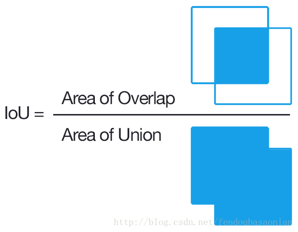
5. IOU (Intersection of Union) in Object Detection

Bounding-box Regression in Object Detection

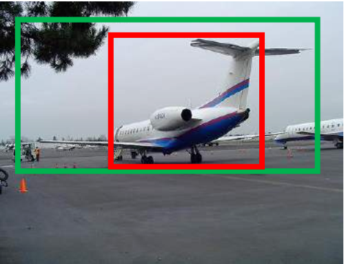
Why do we need Bounding-box Regression? In general, our object detection method predicts bounding-box for an object like blue box in below image. But the groundturth box is shown in green colour, thus we can see the bounding-box of the plane is not accurate compared to the groundtruth box as IOU is lower than 0.5 (intersection of union). If we want to get box location more close to groundtruth, then Bounding-box Regression will help us do this.

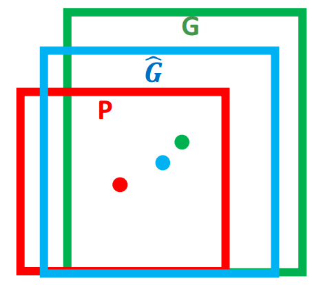
What is Bounding-box Regression? We use $P = (P_x,P_y, P_w, P_y)$ presents the centre coordinates and width/height for the Region Proposals, which is shown as Blue window in the Fig 3. The groundtruth box is represented by $G=(G_x,G_y,G_w,G_h)$. Our aim is to find a projection function $F$ which finds a box $\hat{G}=(\hat{G}_x,\hat{G}_y,\hat{G}_w,\hat{G}_h)$ closer to $G$. In math, we need to find a $F$ which makes sure that $F(P) = \hat{G}$ and $\hat{G} \approx G$.

How to do Bounding-box Regression in R-CNN? We want to transform $P$ to $\hat{G}$, then we need a transformation $(\Delta x, \Delta y, \Delta w, \Delta h)$ which makes the following happen: $$\hat{G}_x = P_x + \Delta x * P_w \Rightarrow \Delta x = (\hat{G}_x - P_x)/P_w$$ $$\hat{G}_y = P_y + \Delta y * P_h \Rightarrow \Delta y = (\hat{G}_y - P_y)/P_h$$ $$\hat{G}_w = P_w e^{\Delta w} \Rightarrow \Delta w = log(\hat{G}_w/P_w)$$ $$\hat{G}_h = P_h e^{\Delta h} \Rightarrow \Delta h = log(\hat{G}_h/P_h)$$

While the groundtruth $(\Delta t_x, \Delta t_y, \Delta t_w, \Delta t_h)$ is defined as: $$\Delta t_x = (G_x - P_x)/P_w$$ $$\Delta t_y = (G_y - P_y)/P_h$$ $$\Delta t_w = log(G_w/P_w)$$ $$\Delta t_h = log(G_h/P_h)$$ Next, we denote $W_i \Phi(P_i)$ where $i \in {x,y,w,h}$ as learned transformation through the neural network, then the loss function is to minimize the L2 distance between $\Delta t_i$ and $W_i \Phi(P_i)$ where $i \in {x,y,w,h}$ by SGD: $$L_{reg} = \sum_{i}^{N} (\Delta t_i - W_i \Phi(P_i))^2 + \lambda ||W||^2$$

6. Upsampling, Deconvolution and Unpooling

Upsampling: upsample any image to higher resolution. It uses upsample and interpolation.

Deconvolution: also called transpose convolution. For example, your input for deconvolution layer is 4x4, deconvolution layer multiplies one point in the input with a 3x3 weighted kernel and place the 3x3 results in the output image. Where the outputs overlap you sum them. Often you would use a stride larger than 1 to increase the overlap points where you sum them up, which adds upsampling effect (see blue points). The upsampling kernels can be learned just like normal convolutional kernels.

Unpooling: We use an unpooling layer to approximately simulate the inverse of max pooling since max pooling is non-invertible. The unpooling operates on following steps: 1. record the maxima positions of each pooling region as a set of switch variables; 2. place the maxima back to the their original positions according to switch variables; 3. reset all values on non-maxima positions to $0$. This may cause some information loss.

Reference:s

1. https://www.quora.com/What-is-the-difference-between-Deconvolution-Upsampling-Unpooling-and-Convolutional-Sparse-Coding

7. RoI Pooling in Object Detection (Fast RCNN)

RoI pooling is simple version of Spatial Pyramid Pooling (multiple division scales, i.e., divide the entire feature maps into (1,4,16) patches/grids), which has only one scale division. For example, the original input image size is (1056x640) and one region proposal ($x_1=0, y_1=80,x_2=245, y_2=498$), after convolutional layers and pooling layers, the feature map size is (66x40), then we should rescale the proposal from ($x_1=0, y_1=80,x_2=245, y_2=498$) to ($x_1=0, y_1=5,x_2=15, y_2=31$) as the scale is 16 (1056/66=16 and 640/40=16). Then we divide the proposal on feature map into 7x7 sections/grids (the proposal size is no need of 7 times) if the output size is 7x7. Next we operate max pooling on each grid, and place the maxima into output 7x7. Here is another simple example below, the input feature size is 8x8, proposal is (0,3,7,8), and the output size is 2x2 thus divide the proposal region into 2x2 sections:

Reference

1. https://zhuanlan.zhihu.com/p/73654026ß

8. RoIAlign Pooling in Object Detection

RoI align Pooling is proposed in Mask RCNN to address the problem that RoI pooling causes misalignments by rounding quantization.

Problem of RoI pooling. There are twice misalignments for each RoI pooling operation. For example, the size of original input image is 800x800, and one region proposal is 515x482 and its corresponding coordinates are ($x_{tl}=20, y_{tl}=267, x_{br}=535, y_{br}=749$) where ‘tl’ means top left and ‘br’ means bottom right. And the stride of last conv layer is **16** which means each feature map extracted from the last conv layer is **50x50** (800/16). If the output size is fixed to 7x7, then RoI pooling would quantize (by floor operation) the region proposal to **32x30** and its corresponding coordinates to ($x_{tl}=1,y_{tl}=16, x_{br}=33, y_{br}=46$). The twice misalignments in each feature map are visualized in the below figure (acutal coordinates in blue colour).

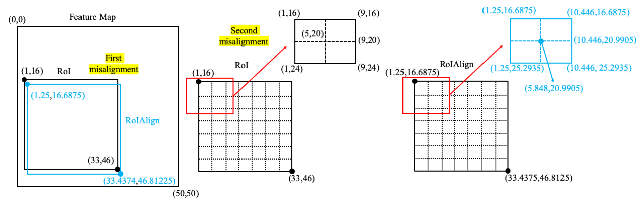
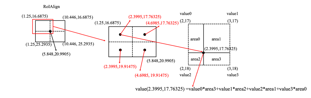
Solution. RoI Align removes all the quantizations of RoI and keeps the float number. Taking the example above, RoI Align Pooling keeps the projected region proposal size 32.1875x30.125 and its corresponding coordinates are ($x_{tl}=1.25,y_{tl}=16.6875, x_{br}=33.4375, y_{br}=46.8125$). Then its corresponding grid size is **4.598x4.303**. We assume the **sample rate is 2**, then 4 points will be sampled. For each grid, we compute the coordinates of 4 sampled points. The coordinates of top left sampled point is (1.25+(4.598/2)/2=2.3995, (16.6875+(4.303/2)/2)=17.76325), the top right sampled point is (1.25+(4.598/2)x1.5=4.6985, 17.76325), the bottom left sampled point is (1.25+(4.598/2)/2=2.3995, 16.6875+(4.303/2)x1.5=19.91475), and the bottom right samples point is (1.25+(4.598/2)x1.5=4.6985, 16.6875+(4.303/2)x1.5=19.91475). For the first sampled point, we compute the value at (2.3995,17.76325) by interpolating values at four nearest points ((2,17),(3,17),(2,18) and (3,18)) in each feature map. The computation of one sampled point can be visualized by the below figure.

where area0=(2.3995-2)x(17.76325-17)=0.304918375, area1=(3-2.3995)x(17.76325-17)=0.458331625, area2=(2.3995-2)x(18-17.76325)=0.094581625, area3=(3-2.3995)x(18-17.76325)=0.142168375.

Reference

1. https://zhuanlan.zhihu.com/p/61317964

9. mAP (mean average precision) in Object Detection

mAP is a measurement metric for the accuracy of object detectors, and it actually computes the mean average precision values along with recall from 0 to 1. Before going deep into mAP, a few concepts should be introduced first, i.e., True Positive, True Negative, False Positive, False Negative, Precision and Recall.

For example, there is a classification task to distinguish whether an image contains apples, then for an image dataset:

True Positive (TP): is how many images containing apples (True) and you predict them contain apples (Positive).

True Negative (TN): is how many images containing apples (True) but you predict them NOT contain apples (Negative).

False Positive (FP): is how many images not containing apples (False) but you predict them contain apples (Positive).

False Negative (FN): is how many images not containing apples (False) and you predict them NOT contain apples (Negative).

Precision: is the percentage of TP among the total number of images that you predict containing apples, which is denoted in math as: $$P = \frac{TP}{TP+FP}$$

Recall: is the percentage of TP among how many images you predict correctly including TP and FN. Correct prediction consists of two parts: 1. you predict an image contains apples and the fact is that it indeed contains apples (this is actually TP); 2. you predict an image not contain apples and the fact is that it indeed not contain apples (this is actually FN). Thus recall is denoted as: $$R = \frac{TP}{TP+FN}$$

9.1 AP

AP is the exact area under the precision-recall curve. In object detection, the prediction is correct if IoU $\geqslant$ 0.5, which means the True Positive is when your prediction satisfies IoU $\geqslant$ 0.5. Then False Positive is IoU < 0.5. For example, if we have a precision-recall curve (red line) like below figure, we first smooth out the zigzag pattern, then at each recall level, we replace each precision value with the maximum precision value to the right of that recall level.

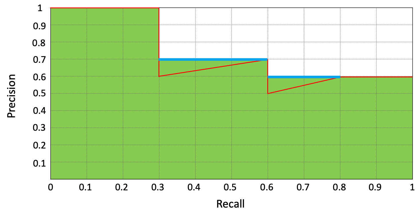
We first smooth out the precision zigzag pattern (recall between 0.3 and 0.6,0.6 and 0.8) by replacing maximum precision value to the right of that recall level (blue line). This happens when the FP number increases first then TP number increases. ($Precision = \frac{TP}{TP+FP}$, FP $\uparrow$, Precision $\downarrow$. TP $\uparrow$, Precision $\uparrow$. ). Then $AP = \frac{1}{10}(1 \times 3 + 0.7 \times 3 + 0.6 \times 4)=0.75$ (green area).

mAP is the average of AP. In some context, we compute the AP for each class then average them. But in some context, they mean the same thing. For example, in COCO context, AP is averaged over all categories, which means there is no difference between mAP and AP.

Reference

https://medium.com/@jonathan_hui/map-mean-average-precision-for-object-detection-45c121a31173

10. Cross Validation

10.1 Model vs Learner

Model is general a mapping function from input to output, and it could be a machine learning algorithm (e.g., Logistic regression/SVM) or deep neural network (e.g., CNN/GCN/GAN). While Learner is general a model with learned weights which is a learned model after training.

10.2 Hyperparameters vs parameters in Model

Hyperparameters are the user pre-defined parameters of a model before training (e.g., learning-rate), while parameters are the learned weights after training, for example, $w^T$ in linear regression $f(x) = w^T x + b$.

10.3 K-fold Cross Validation

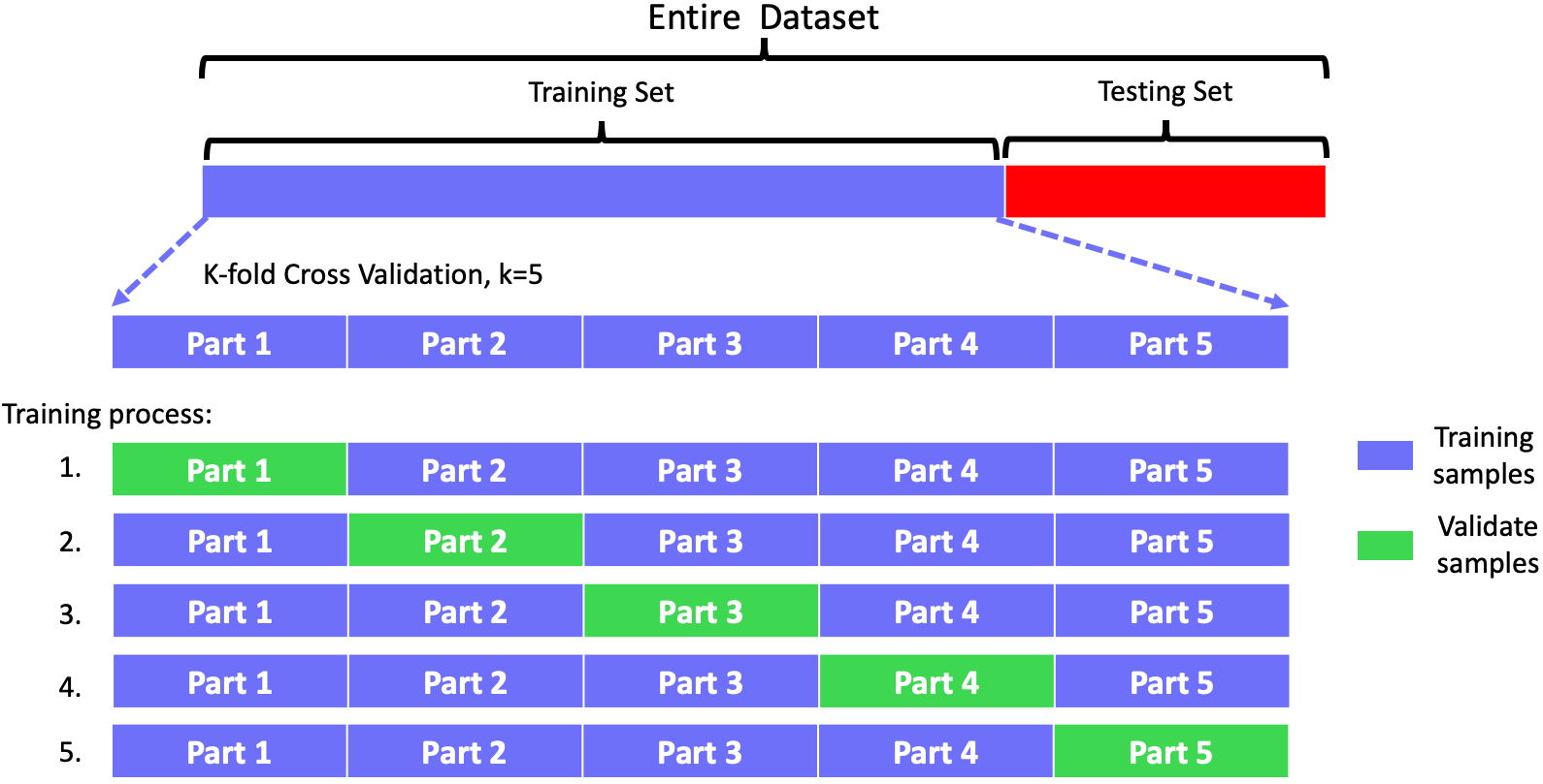
Given a dataset, we first divide it into training set and testing set which is not accessible to model during training stage. Then we further divide the training set into a training part and a validate part by k-fold cross validation.

For example, if we choose $k=5$ then the training set will be divided into 5 parts of equal size, like part 1, part 2, part 3, part 4 and part 5. During training, we take part 1 as validate samples and the rest as true training samples, which means the model will be trained with the part 2-4 and validated by part 1. Then we choose part 2 as validate samples and the rest as true training samples, which means the model will be trained with part1,3-5 and validated by part 2. Continue, until each part has been chosen as validate samples. Thus this process is repeated $k=5$ times. After this, the model has been trained with all the samples of the training set (though it is not in once time). Then we use mean of mean square error: $$cv_{k} = \frac{1}{k} \sum_{i=1}^k MSE(x_i)$$ to see the cross validate score. The illustration is as follow:

References

https://zhuanlan.zhihu.com/p/24825503

11 Why do Variational Autoencoders (VAE) compute KL divergence loss?

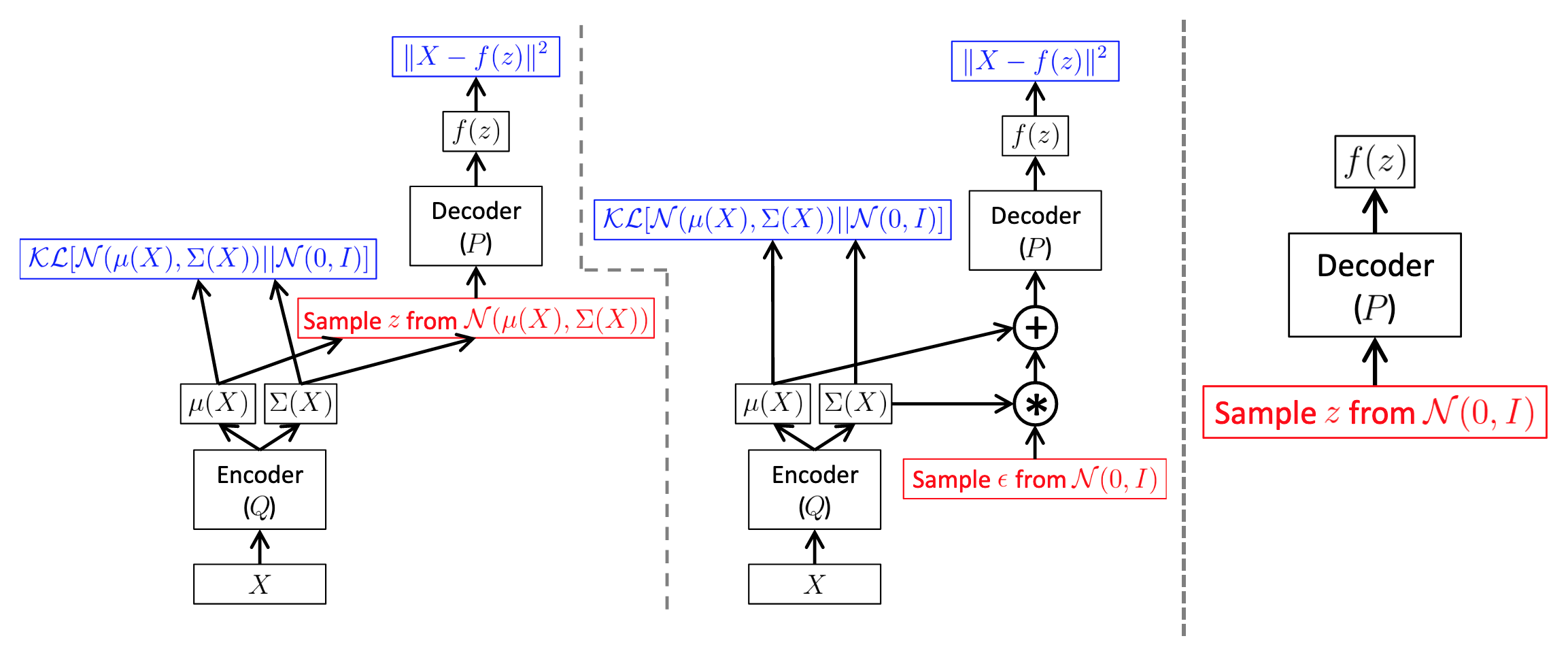
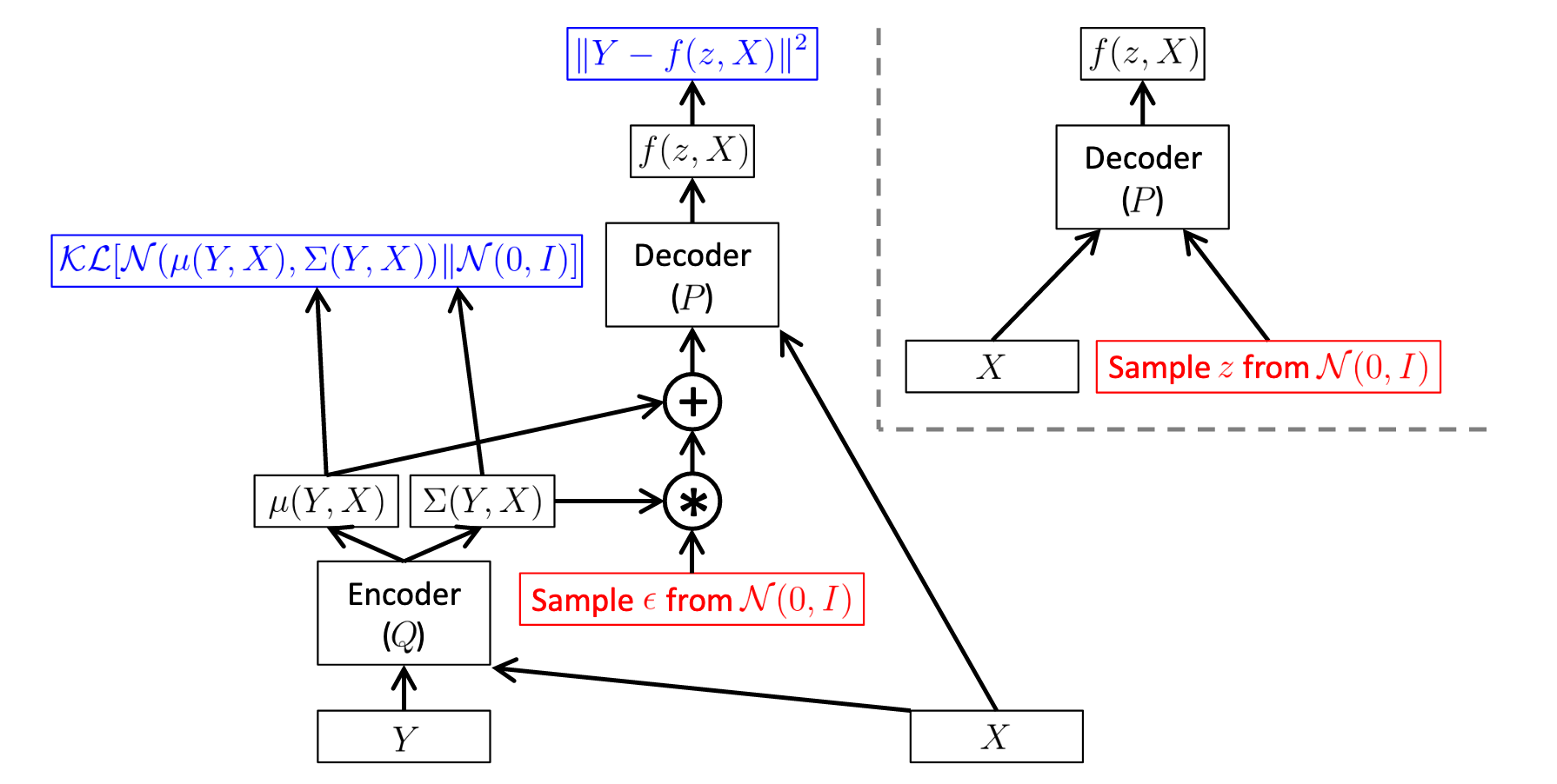
Variational autoencoders aim to map the input data into a distribution (aka latent vector) instead of just a fixed vector, as once the model is learned we can generate arbitrary output by just sampling from this learnt distribution. In this way, during test time, we can discard the encoder part and just use the decoder to produce new outputs that are not seen in training set. However, in general cases, the distribution of learned latent vector could be variant to inputs in training dataset. To address this problem, we assign the learned distribution of latent vectors to be a Gaussian distribution, then we sample arbitrary $z$ from this distribution and produce new outputs by passing $z$ into the decoder. To enforce the learned distribution, we use Kullback-Leibler (KL) divergence loss to emphasize the distribution distance between learned distribution and Gaussian distribution.

During the training-time, a variational autoencoder implemented as a feed-forward neural network, where $P(X|z)$ is Gaussian. Left is without the “reparameterization trick”, and right is the with it. Red shows sampling operation is non-differentiable. Blue shows loss layers. The feed-forward behaviour of these networks is identical, but backpropagation can be applied only to the right network. This KL divergence loss is to promote Gaussian distribution in the latent space. Regularly, there should also be a regularization term (i.e., $l_2$ norm) which is used to avoid overfitting.

For a conditional variational autoencoder, we hope the autoencoder could produce some plausible outputs with additional input (aka condition). For example, we want an MINST digit autoencoder could produce a digit just like a particular person’s writing or style. In figure 10, left is a training-time conditional variational autoencoder implemented as a feefforward nerual network, following the same notation as Fig 9. Right is same decoder at test time, where $X$ denotes the condition in both training and testing time.

Reference

1. https://arxiv.org/pdf/1606.05908.pdf
2. https://lilianweng.github.io/lil-log/2018/08/12/from-autoencoder-to-beta-vae.html