EfficientNet_mobilenet_shufflenet

1. Background

In this post, we use the following symbols for all sections:

1. $W$: width, $H$: height
2. $N$: input channel, $M$: output channel
3. $K$: convolution kernel size.

1.1 Params for a neural network

Params is related to the model size, the unit is Million in float32, thus the model size is approximately 4 times of params. For a standard convolution operation, the params = $(K^2 \times N + 1)M$, without bias: $K^2 \times NM$. For a standard fully connection layer, the params = $(N+1)M$, without bias: $NM$.

1.2 Computation complexity (FLOPs)

Computational complexity (or cost) is related to speed (but indirect), and it is usually written as FLOPs. Here only multiplication-adds is considered. For a standard convolution operation, the FLOPs = $WHN \times K^2M$. For a fully connection layer, the FLOPs = $(N+1)M$, without bias: $NM$. Here we can see that the FLOPs is nearly $WH$ times of Params for a conv operation.

1.3 Compute the params and FLOPs in PyTorch

In pytorch, opCounter library can be used to compute the params and FLOPs of a model. Install opCouter first:

pip install thop

For instance, computing these numbers can be done by following code:

from torchvision.models import resnet50
from thop import profile

model = resnet50()
input = torch.randn(1,3,224,224)
flops, params = profile(model, inputs=(input,))

2. Computational cost for convolution layers

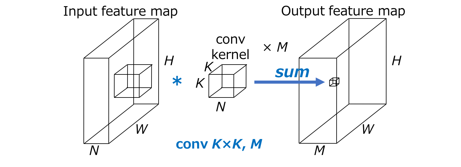
We will check on the computation of a general convolution operation. For example, in Fig 1, the input feature has the dimensions like width $W$ $\times$ height $H$ $\times$ N (input channels), the convolution kernel has dimension like $K \times K$ (kernel size) $\times$ M (output channels) and the convolutional operation has stride=1 and padding=1 which keeps the width and height same between input and output, thus the output feature will have the dimension $W \times H \times M$. Then the multiply-add computation (standard computational cost) of a general conv operation is $WHN \times K^2 M$.

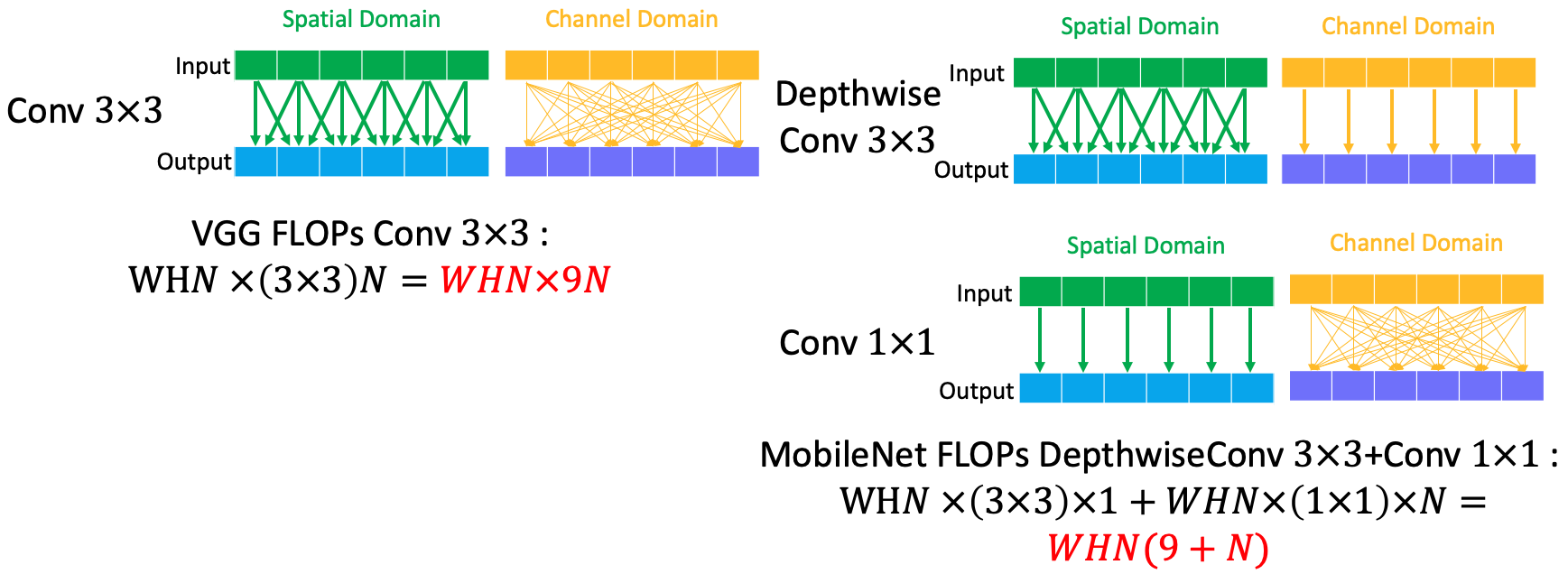
2.1 Computation cost of conv $3 \times 3$ and conv $1 \times 1$

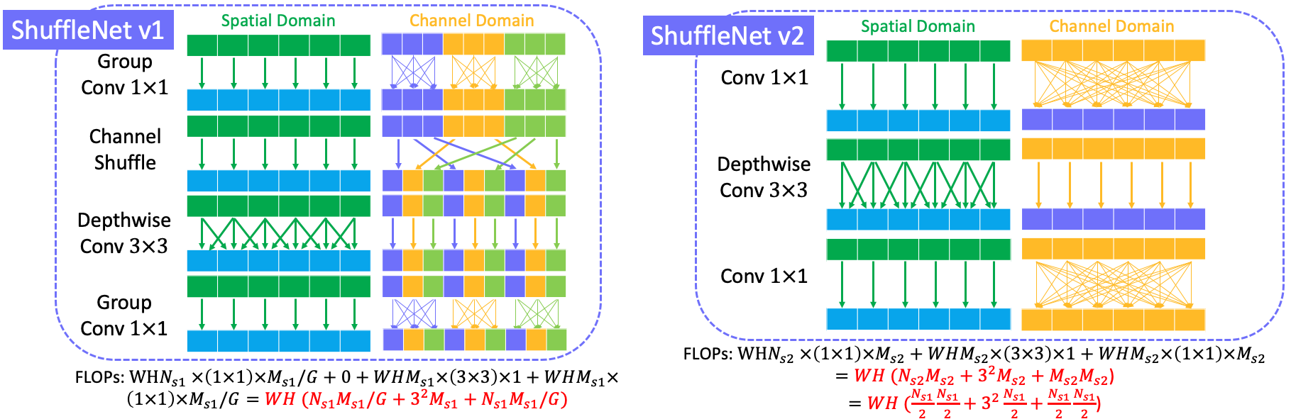
Normally, the most used conv kernel in modern neural network is $3 \times 3$, which is denoted as conv $3 \times 3$. Its computational cost is $WHN3^2M$ when the convolution operates on both spatial and channel domain. If we illustrate the computation cost on spatial and channel domain, the following fig could be a better visualization. We can there is a fully connection between input channels and output channels.

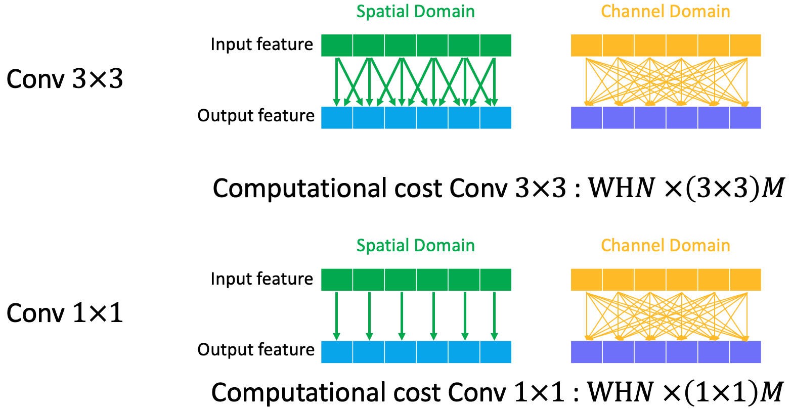
For conv $1\times1$, the spatial connect is $1\times1$ linear projection while channel projection is still fully connected, which leads to computational cost $WHN \times 1^2 M$. Compared to conv $3 \times 3$, the computation is reduced by $\frac{1}{K^3} = \frac{1}{9}$ in this case.

2.2 Computation cost of group convolution

Group convolution is firstly introduced in AlexNet to deal with the insufficient GPU memory and, to some extent, reduce the learned number of parameters. Grouped convolution operates on channel domain, which divides the channels into $G$ groups and the information in different groups is not shared. In each group, the connection still follows the fully connection way. The computation costs for grouped conv $3\times3$ and conv $1\times1$ are as following:

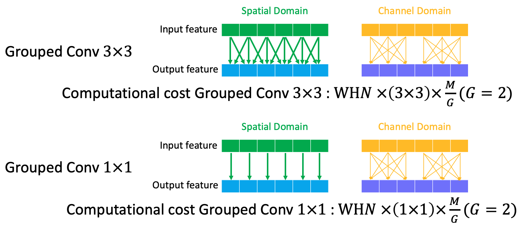
Compared to standard conv, the grouped conv $3\times3$ (where $G=2$) reduce the connection in channel domain by factor $G$, which results in $\frac{1}{G}$ times of standard conv.

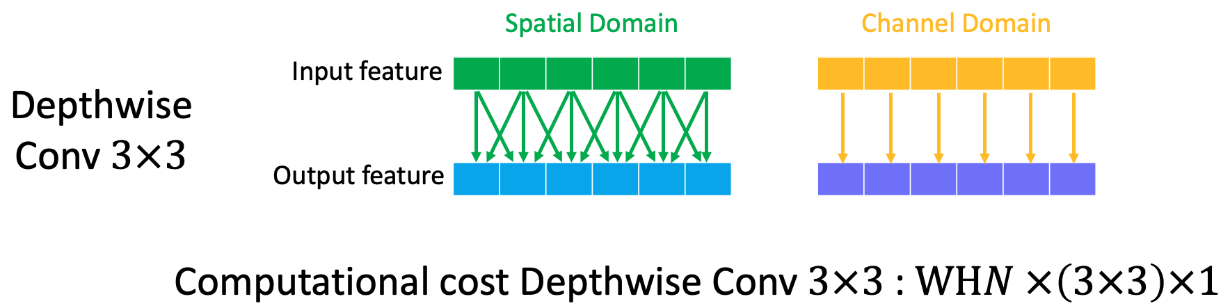
2.3 Computation cost of depthwise convolution

Depthwise convolution is firstly introduced in MobileNet v1, which performs the convolution operation independently to for each of input channels. Actually, this can be regarded as a special case of grouped conv when $G=N$. Usually, output channel $M » K^2$, thus depthwise conv significantly reduces the computational cost compared to standard conv operation.

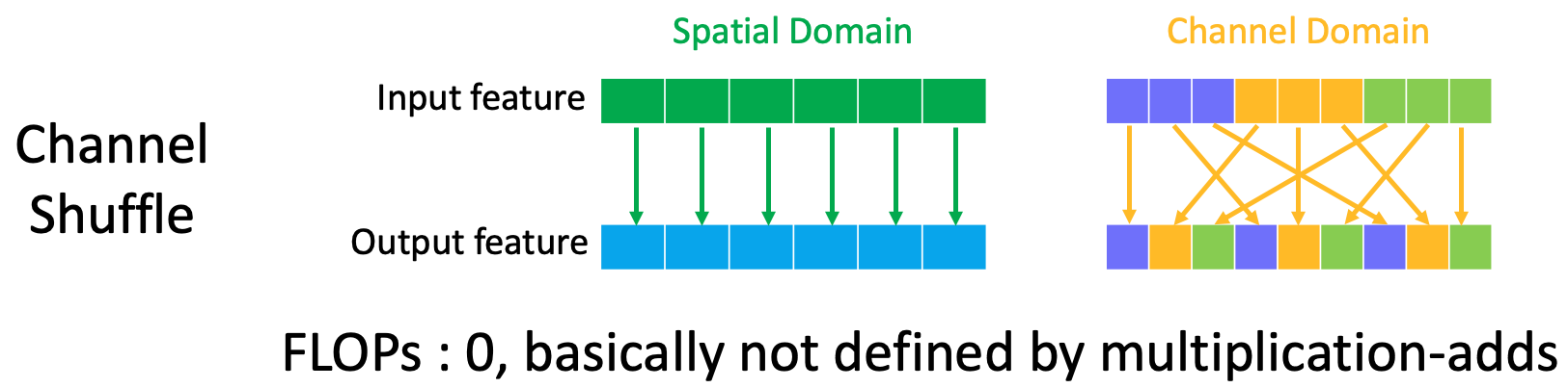
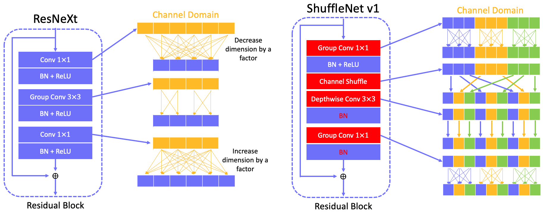
2.4 Channel shuffle

Channel shuffle is an operation introduced in ShuffleNet v1 to deal with the large computational cost by conv $1\times1$ in ResNeXt network. In this section, we basic show how channel shuffle works and introduce more details in Section 5. The operation is first divide the input channels $N$ into $G$ groups, which results in $G \times N^{`}$ channels. Usually, the $N^{`}$ is a certain times of $G$. In this case, $N^{`}=9$ and $G=3$. Then one certain channel in a group will stay in the same group, but each of the rest channel in a group will be separately assigned to other groups. The figure below illustrates the channel shuffle operation.

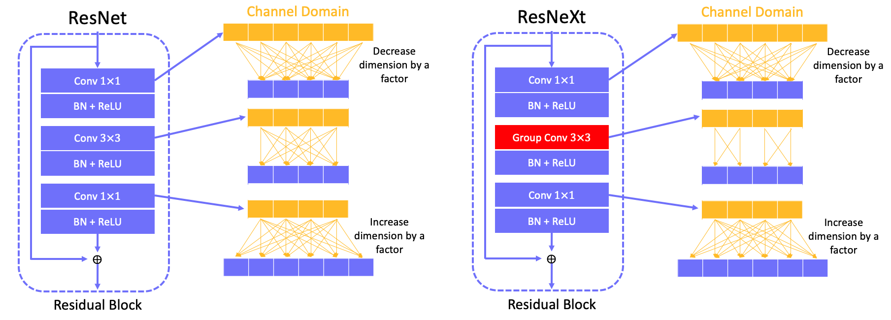
3. ResNet, ResNeXt

3.1 Bottleneck architecture comparison

Basic idea in ResNeXt is to replace standard conv $3\times3$ by group conv $3\times3$.

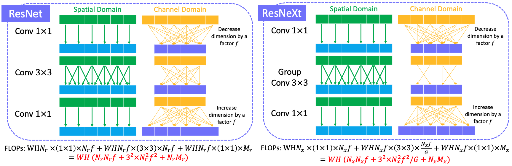
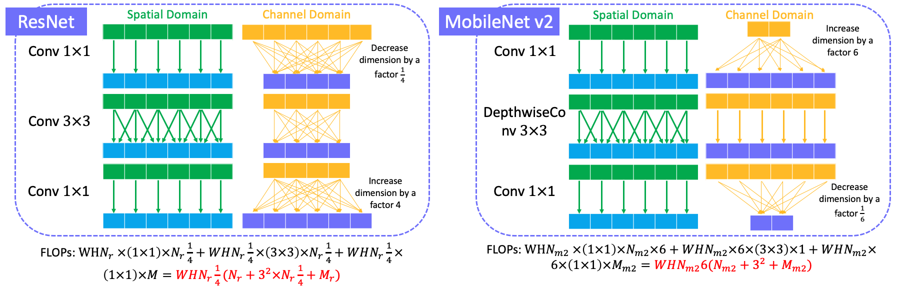
3.2 FLOPs comparison

Note that FLOPs of ResNeXt is only reduced by a small budget of computational cost and it’s up to group number $G$ when $N_r=N_x$ and $M_r=M_x$.

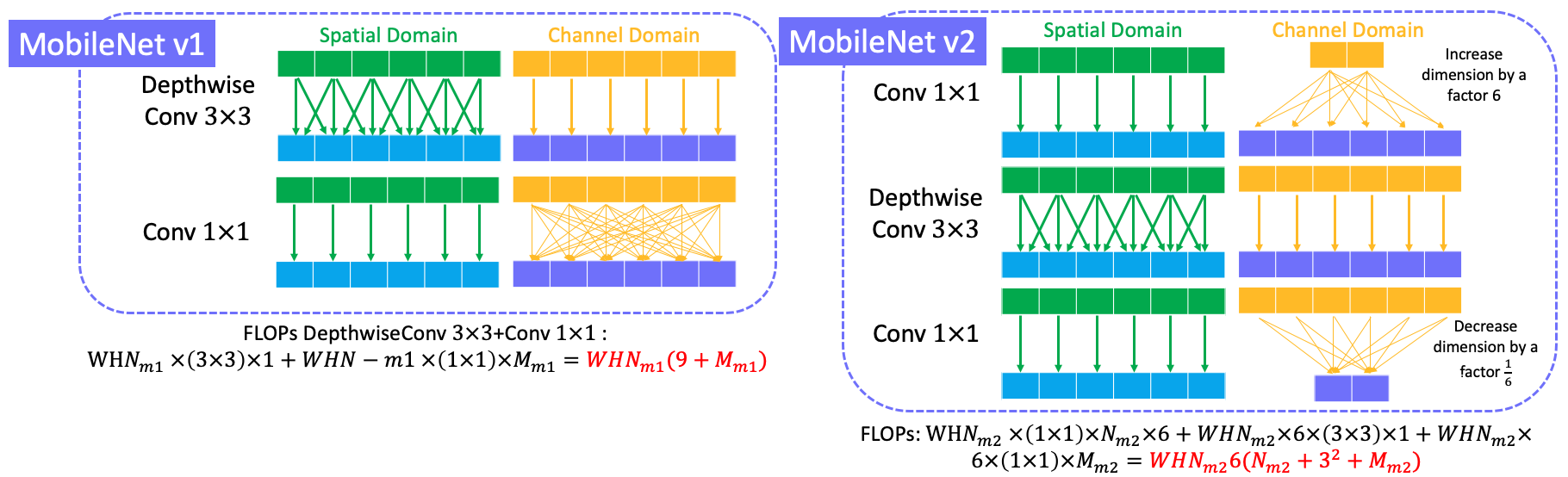
4. MobileNet v1 vs v2

4.1 MobileNet v1 (VGG)

Key point is to replace all standard conv $3\times3$ with depthwise conv $3\times3$ + conv $1\times1$ in standard VGGNet. This blog says that the ReLU is also replaced by ReLU6 (ReLU6 = $max(max(0,x),6)$) in MobileNet v1, but the original paper does not say anything about it. Perhaps in engineering projects, people usually use ReLU6.

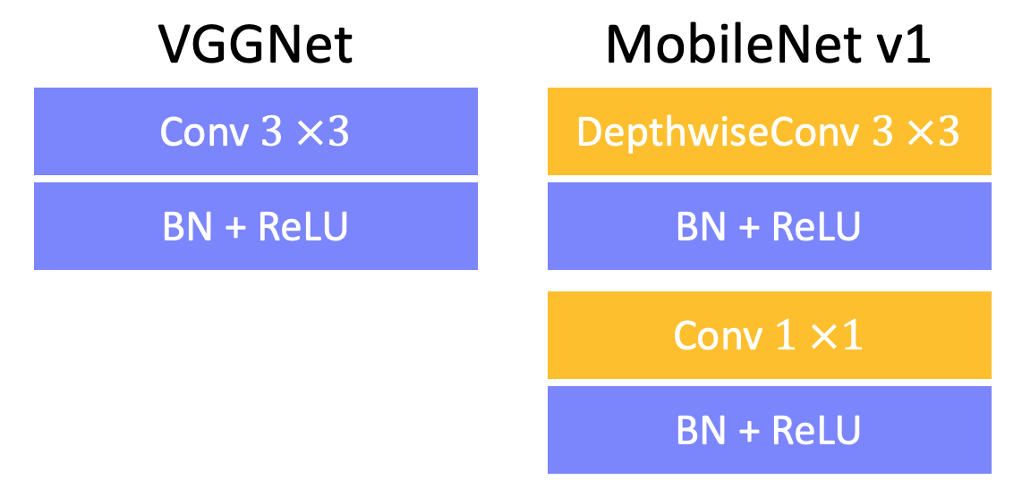
Therefore, the FLOPs is reduced about $\frac{1}{8}$ ~ $\frac{1}{9}$ in MobileNetv1 compared to VGGNet.

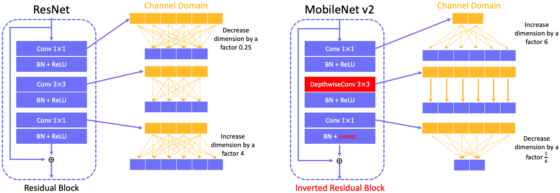
4.2 MobileNet v2 (ResNet)

Key point is to replace the last ReLU with linear bottleneck and introduce an inverted residual block in ResNet. The reason behind of replacing relu with a linear transformation is that relu causes much information loss when input dimension is low. The inverted residual block consists of a conv $1\times1$ (expanse low dimension input channels to high dimension channels) + a depthwiseconv $3\times3$ + a conv $1\times1$ (decrease high dimension input channels to low dimension (original) channels).

Inverted residual block in Mobilenet v2 (see figure 9). Only the last ReLU is replaced by a linear transformation, because the input dimensions of conv $1\times1$ and depthwise conv $3\times$ are increased compared to original dimension, thus relu works fine. But when the input dimension is decreased by the last conv $1\times1$, relu will lose much information, thus we replace relu with a linear transformation to preserve as much as original information.

Here we compute the FLOPs for a standard residual block in ResNet and an inverted residual block in MobileNet v2. As can be seen, when the ResNet input channel $N_r$ and output channel $M_r$ is equal to MobileNet v2 input channel $N_{m2}$ and output channel $M_{m2}$, MobileNet v2 has a larger FLOPs than ResNet. However, the advantage of MobileNet v2 is that it only needs a much smaller input channel and output channel while achieves similar accuracy of ResNet, which eventually leads to smaller FLOPs than ResNet.

4.3 Comparison

Here shows the convolution block in MobileNet v1 and v2, and their FLOPs comparison.

Note that the FLOPs for a single inverted residual block has an extra term ($N_{m2}$) as there is an extra conv $1\times1$ used compared to MobileNet v1. However, MobileNet v2 still has smaller params and FLOPs than MobileNet v1 as the input channel $N_{m2}$ and output channel $M_{m2}$ could be smaller than $N_{m1}$ and $M_{m1}$ of MobileNet v1. Please refer to Table 3 in original MobileNet v2 paper for more details.

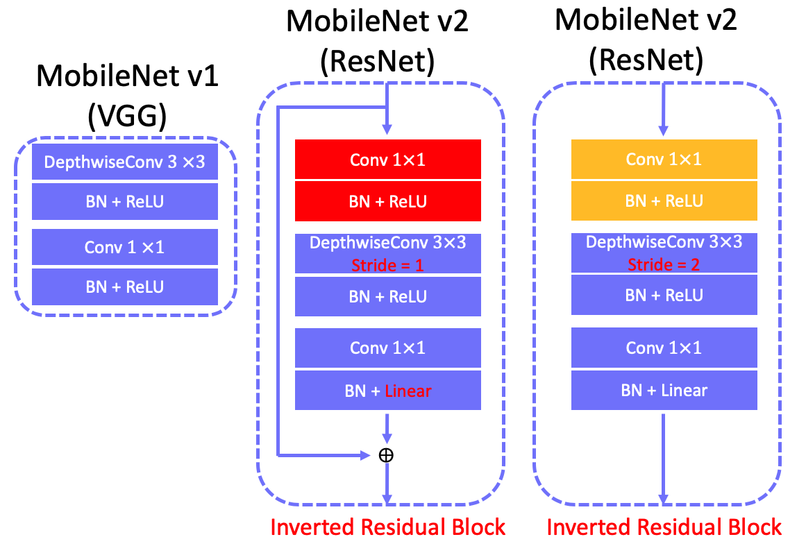
Why MobileNet v2 is not faster than MobileNet v1 on Desktop computer? On desktop, the separable depthwise convolution is not directly supported in GPU firmware (cuDNN library). While MobileNet v2 could be slightly slower than MobileNet v1 as V2 has more separable depthwise convolution operations and more larger input channels (96/192/384/768/1536) of using separable depthwise convolution than V1 (64/128/256/512/1024).

Why MobileNet is not as fast as FLOPs indicates in practice? One reason could be the application of memory takes much time (according to some interviews).

5. ShuffleNet v1 vs v2

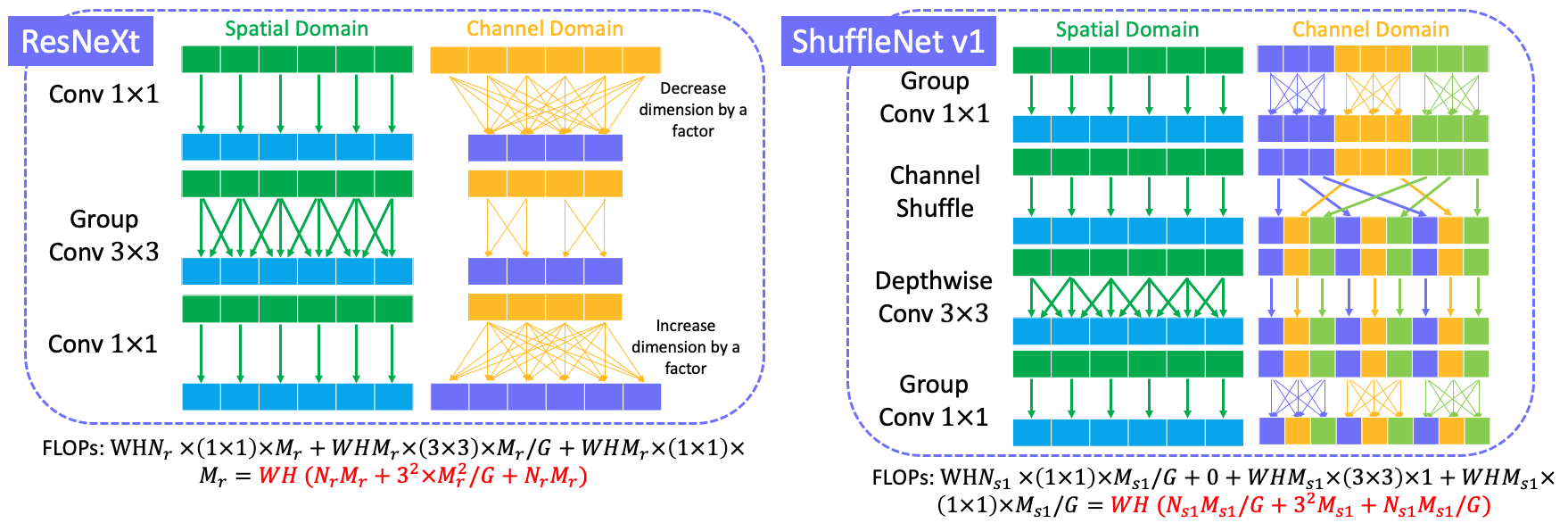
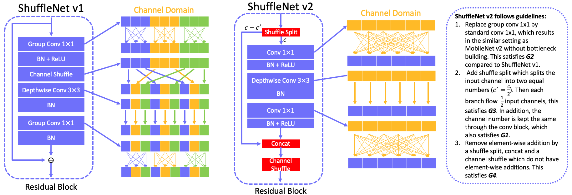
5.1 ShuffleNet v1 (ResNeXt)

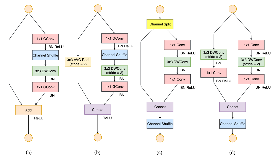
ResNeXt is an efficient model for ResNet by introducing group conv $3\times3$ to reduce computational cost. However, the computational cost of conv $1\times1$ become the operation consuming most of time. To reduce the FLOPs of conv $1\times1$, ShuffleNet v1 introduce group conv $1\times1$ tp replace the standard conv $1\times1$. However, the features won’t be shared between groups by using group conv $1\times1$, which causes less feature reuse and accuracy. To address this problem, a channel shuffle operation is introduced to share features between groups. The basic blocks of ResNeXt and ShuffleNet v1 is shown in the below figure.

Here we also give the computational cost of each method:

ResNeXt FLOPs = $WH(2N_r M_r + 9M_r^2/G)$

ShuffleNet v1 FLOPs = $WH(2N_{s1}M_{s1}/G + 9M_{s1})$, where $G$ is the group number.

It is obviously that ShuffleNet v1 FLOPs < ResNeXt FLOPs when $N_r=N_{s1}$ and $M_r = M_{s1}$.

5.2 ShuffleNet v2

ShuffleNet v2 points out that FLOPs is an indirect metric to evaluate computational cost of a model since the run time should also contain the memory access cost (MAC) , degree of parallelism and even hardware platform (e.g., GPU and ARM). Thus shufflenet v2 introduces a few rules to evaluate the computational cost of a model by considering the factors above.

5.2.1 Guidelines for evaluating computational cost

• G1. MAC is minimal when input channel is equal to output channel. Let $WHN$ denote input feature, $WHM$ be output feature. Then FLOPs $F=WHNM$ when conv kernel is $1\times1$. We simply assume that input feature occupies $WHN$ memory, output feature occupies $WHM$ memory, and conv kernels occupy $NM$ memory. Then MAC can be denoted as: \begin{eqnarray} MAC &=& WHN + WHM +NM \\\
  &=& WH(N+M) + NM \\\
  &=& \sqrt{(WH)^2(N+M)^2} + \frac{F}{WH} \\\
  &\geqslant& \sqrt{(WH)^2\times 4NM} + \frac{F}{WH} \\\
  &=& \sqrt{(WH)\times 4WHNM} + \frac{F}{WH} \\\
  &=& \sqrt{(WH)\times 4F} + \frac{F}{WH} \\\
  \end{eqnarray} Thus MAC achieves the minimal value when input channel $N$ is equal to output channel $M$ under same FLOPs.
• G2. MAC increases when the number of group increases. FLOPs $F=WH \times N \times M/G$. Then MAC is denoted as: \begin{eqnarray} MAC &=& WHN + WHM + \frac{NM}{G} \\\
  &=& F\times \frac{G}{M} + F \times \frac{G}{N} + \frac{F}{WH} \\\
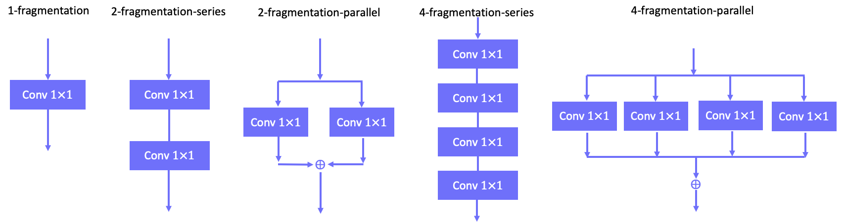
  \end{eqnarray} Thus MAC increase with the growth of $G$.
• G3. Network fragmentation reduces degree of parallelism. More fragmentation causes more computational cost in GPU. For example, under the same FLOPs, the computation efficiency is as following order: 1-fragmentation > 2-fragmentation-series > 2-fragmentation-parallel > 4-fragmentation-series > 4-fragmentation-parallel.

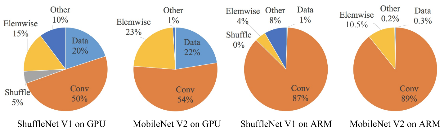
• G4. Element-wise operations consume much time. Except convolution operations, the element-wise operation is the second operation consuming much time.

Based on the guidelines above, we can analyse that shufflenet v1 introduces group convolutions which is against G2, and if it uses bottleneck-like blocks (using conv$1\times1$ change input channels) then it is against G1. MobileNet v2 introduces an inverted residual bottleneck which is against G1. And it uses depthwise conv $3\times3$ and ReLU on expansed features and leads to more element-wise operation which violates G4. The autogenerated structures (searched network) add more fragmentations which violates G3.

5.2.2 ShuffleNet v2 architecture

Following the guidelines in aforementioned section, shufflenet v2 introduces their new version of shufflenet.

Since the channel split, concat and channel shuffle are basically not multiplication-adds operations, the FLOPs is computed in the block inside. Note that $N_{s2}=M_{s2}=\frac{N_{s1}}{2}$, thus shuffleNet v2 is more efficient than ShuffleNet v1 ($G=4$) even under FLOPs evaluation.

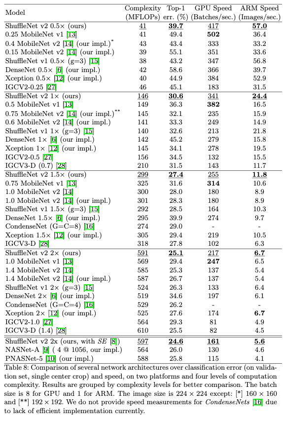
5.3 Comparison to other state-of-the-art methods

5.2.3 One more thing

ShuffleNet v2 shares the similar idea with DenseNet that is strong feature reuse, which makes ShuffleNet v2 achieve similar high accuracy as DenseNet but in a more efficient manner. More recently, a CondenseNet (upgraded DenseNet) points out that the more short distance features the more important they are to current layer features. Similar to Condensenet, feature map at $j$-th bottleneck building in ShuffleNet v2 reuses $\frac{c_i}{2^{j-i}}$ of feature maps at $i$-th bottleneck building, which reuses more feature maps when $j$ is more close to $i$.

Reference:

1. https://zhuanlan.zhihu.com/p/37074222
2. https://medium.com/@yu4u/why-mobilenet-and-its-variants-e-g-shufflenet-are-fast-1c7048b9618d
3. https://zhuanlan.zhihu.com/p/51566209
4. https://cloud.tencent.com/developer/article/1461275