Graph_NN
This blog simply clarifies the concepts of graph embedding, graph neural networks and graph convolutional networks.
Graph Embedding
Graph Embedding (GE) is in representation learning of neural network, which often contains two types:
- embed each node in a graph into a low-dimension, scalar and dense vector, which can be represented and inferenced for learning tasks.
- embed the whole graph into a low-dimension, scalar and dense vector, which can be used for graph structure classification.
There are three types of method to complete graph embedding:
- Matrix Factorization. A representable matrix of a graph is factorized into vectors, which can be used for learning tasks. The representable matrix of a graph are often adjacency matrix, laplacian matrix etc.
- Deepwalk. Inspired by word2vec, the deepwalk considers the reached node list by random walk as a word, which is fed into word2vec network to obtain a embeded vector for learning tasks.
- Graph Neural Network. It is basically a series of neural networks operating on graphs. The graph information like representable matrix is fed into neural networks in order to get embedded vectors for learning tasks.
Graph Neural Networks
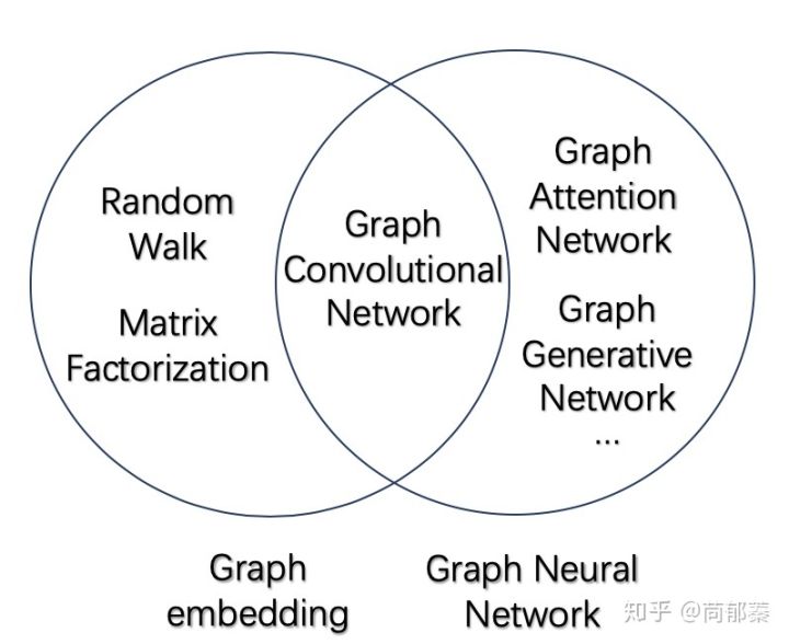
Graph Neural Networks (GNN) are deep neural networks with graph information as input. In general, the GNN can be divided into different types: 1. Graph Convolutional Networks (GCN); 2. Graph Attention Networks (GAT); 3. Graph Adversarial Networks; 4. Graph LSTM. The basic relationship between GE, GNN,GCN is shown as following picture:
Graph Convolutional Networks
Graph Convolutional Networks (GCN) operate convolution on graph information like adjacency matrix, which is similar to convolution on pixels in CNN. To better clarify this concept, we will use equations and pictures in the following paragraph.
Concepts
There are two concepts should be understood first before GCN. Degree Matrix (D): this matrix ($N \times N$, N is the node number) is a diag matrix in which values in diag line means the degree of each node; Adjacency Matrix (A): this matrix is also a $N \times N$ matrix in which value $A_{i,j}=1$ means there is an edge between node $i$ and $j$, otherwise $A_{i,j}=0$;
Simple GCN example
Let’s consider one simple GCN example, which has one GCN layer and one activation layer, the formulation is as following: $$f(H^{l}, A) = \sigma(AH^{l}W^{l})$$ where $W^l$ denotes the weight matrix in the $l$th layer and $\sigma(\dot)$ denotes the activation function like ReLU. This is the simplest expression of GCN example, but it’s already much powerful (we will show example below). However, there are two basic limitations of this simple formulation:
- there is no node self information as adjacency matrix $A$ does not contain any information of nodeself.
- there is no normalization of adjacency matrix. The formulation $AH^{l}$ is actually a linear transformation which scales node feature vectors $H^l$ by summing the features of all neighbour nodes. The nodes having more neighbour nodes has more impact, which should be normalized.
Fix limitation 1. We introduce the identity matrix $I$ into adjacency matrix $A$ to add nodeself information. For example, $\hat{A} = A + I_n$ where $I_n$ is the identity matrix with $n \times n$ size.
Fix limiation 2. Normalizing $A$ means that all rows of $A$ should sum to be one, and we realize this by $D^{-1}A$ where $D$ is the diag degree matrix. In practise, we surprisingly find that using a symmetric normalization, e.g., $D^{-\frac{1}{2}}AD^{-\frac{1}{2}}$ is more dynamically more interesting (I still do not get it why use symmetric normalization $D^{-\frac{1}{2}}AD^{-\frac{1}{2}}$). Combining these two tricks, we get the propagation rule introduced in Kipf et al. 2017: $$f(H^l, A) = \sigma(\hat{D}^{-\frac{1}{2}}\hat{A}\hat{D}^{-\frac{1}{2}}H^lW^l)$$ where $\hat{A} = I_n + A$ and $\hat{D}$ is the diagonal node degree matrix of $\hat{A}$. In general, whatever matrix multiplies $H^lW^l$ (i.e. $A$, $D^{-1}A$ or $\hat{D}^{-\frac{1}{2}}\hat{A}\hat{D}^{-\frac{1}{2}}$) is called Laplacian Matrix, which can be denoted as $L_{i,j}$ the value for $i$th and $j$th node. Taking the laplacian Matrix introduced in Kipf et al. 2017 as an example, the $L_{i,j}$ is as following: \begin{equation} L_{i,j}^{sym} = \begin{cases} 1, &i=j, deg(j) \neq 0 \newline -\frac{1}{\sqrt{deg(i)deg(j)}}, &i \neq j, j \in \Omega_i \newline 0, &otherwise \end{cases} \end{equation} where deg($\cdot$) denotes the degree matrix and $\Omega_i$ denotes all the neighbour nodes of node $i$. This symmetric Laplacian matrix not only considers the degree of node $i$ but also takes the degree of its neighbour node $j$ into account, which refers to symmetric normalization. This propagation rule weighs neighbour in the weighted sum higher if the node $i$ has a low-degree and lower if the node $i$ has a high-degree. This may be useful when low-degree neighbours have bigger impact than high-degree neighbours.
Code example for simple GCN
Considering the following simple directed graph:
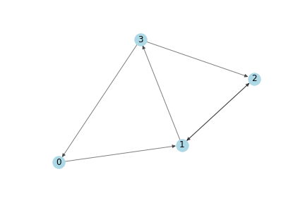
Then the Adjacency Matrix $A$ is:
A = np.matrix([
               [0.,1.,0.,1.],
               [0.,0.,1.,1.],
               [0.,1.,0.,0.],
               [1.,0.,1.,0.]],
               dtype=float)
the identity matrix $I_n$ of $A$ is:
I_n = np.matrix([
              [1.,0.,0.,0.],
              [0.,1.,0.,0.],
              [0.,0.,1.,0.],
              [0.,0.,0.,1.]],
              dtype=float)
We assign random weight matrix of one GCN layer:
W = np.matrix([[1,-1],[-1,1]])
Next we randomly give 2 integer features for each node in the graph.
H = np.matrix([[i,-i] for i in range(A.shape[0])], dtype=float)
H
matrix([[ 0.,  0.],
        [ 1., -1.],
        [ 2., -2.],
        [ 3., -3.]])
Now the unnormalized features $\hat{A}H$ are:
A_hat * H
matrix([[ 1., -1.],
        [ 6., -6.],
        [ 3., -3.],
        [ 5., -5.]])
the output of this GCN layer:
A_hat * H * W
matrix([[  2.,  -2.],
        [ 12., -12.],
        [  6.,  -6.],
        [ 10., -10.]])
# f(H,A)=relu(A_hat * H * W)
relu(A_hat * H * W)
matrix([ [2., 0.],
         [12.,0.]
         [6., 0.],
         [10., 0]])
Next we apply the propagation rule introduced in Kipf et al. 2017. First, we add self-loop information $\hat{A} = A + I$ is :
A_hat = A + I_n
A_hat
matrix([
      [1.,1.,0.,0.],
      [0.,1.,1.,1.],
      [0.,1.,1.,0.],
      [1.,0.,1.,1.]])
Second, we add normalization by computing $\hat{D}$ and $\hat{D}^{-\frac{1}{2}}$ (inverse matrix of square root of $\hat{D}$):
D_hat = np.array(np.sum(A_hat, axis=0))[0]
D_hat = np.matrix(np.diag(D_hat))
D_hat
matrix([[ 2.,  0.,  0.,  0.],
        [ 0.,  3.,  0.,  0.],
        [ 0.,  0.,  3.,  0.],
        [ 0.,  0.,  0.,  2.]])
inv_D_hat_sqrtroot = np.linalg.inv(np.sqrt(D_hat))
inv_D_hat_sqrtroot
matrix([[ 0.70710678,  0.        ,  0.        ,  0.        ],
        [ 0.        ,  0.57735027,  0.        ,  0.        ],
        [ 0.        ,  0.        ,  0.57735027,  0.        ],
        [ 0.        ,  0.        ,  0.        ,  0.70710678]])
Next, we compute the Laplacian matrix of $L = \hat{D}^{-\frac{1}{2}}\hat{A}\hat{D}^{-\frac{1}{2}}$ and the nomalized features $L * H$ :
Laplacian_matrix = inv_D_hat_sqrtroot * A_hat * inv_D_hat_sqrtroot
Laplacian_matrix
matrix([[ 0.5       ,  0.40824829,  0.        ,  0.        ],
        [ 0.        ,  0.33333333,  0.33333333,  0.40824829],
        [ 0.        ,  0.33333333,  0.33333333,  0.        ],
        [ 0.5       ,  0.        ,  0.40824829,  0.5       ]])
# normalized feature vectors
Laplacian_matrix * H
matrix([[ 0.40824829, -0.40824829],
        [ 2.22474487, -2.22474487],
        [ 1.        , -1.        ],
        [ 2.31649658, -2.31649658]])
#non-normalized feature vectors
A_hat * H
matrix([[ 1., -1.],
        [ 6., -6.],
        [ 3., -3.],
        [ 5., -5.]])
As can be seen, all the values of feature vectors are scaled to smaller absolute values than Non-normalized feature vectors.
Finally, the output of GCN layer with applying the propagation rule:
# f(H,A) = relu(L*H*W)
relu(Laplacian_matrix*H*W)
matrix([[ 0.81649658, 0.],
        [ 4.44948974, 0.],
        [ 2.        , 0.],
        [ 4.63299316, 0.]])
# compared to f(H,A) = relu(A_hat*H*W)
relu(A_hat*H*W)
matrix([[  2.,  0.],
        [ 12.,  0.],
        [  6.,  0.],
        [ 10., 0.]])
I suggest to verify this operation by yourself.
Real example: Semi-Supervised Classification with GCNs
Kipf & Welling ICLR 2017 demonstrates that the propgation rule in GCNs can predict semi-supervised classification for social networks. In this semi-supervised learning example, we assume that we know all the graph information including nodes and their neighbours, but not all the node labels, which means some nodes are labeled but others are not labeled.
We train the GCNs on labeled nodes and propagate the node label information to unlabedled nodes by updating weight matrices shared arcoss all nodes. This is done by following steps:
- perform forward propagation through the GCN layers.
- apply sigmoid function row-wise at the last layer of GCN.
- compute the cross entropy loss on known node labels.
- backpropagate the loss and update the weight matrices $W$ in each layer.
Zachary’s Karate Club
Zachary’s Karate Club is a typical small social network where there are a few main class labels. The task is to predict which class each member belongs to.
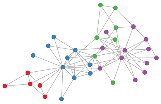
We run a 3-layer GCN with randomly initialized weights. Now before training the weights, we simply insert Adjacency matrix $A$ and feature $H=I$ (i.e., $I$ is the identity matrix) into the model, then perform three propagation steps during the forward pass and effectively convolves the 3rd-order neighbourhood of each node. The model already produces predict results like picture below without any training updates:
Now we rewrite the propagation rule in layer-wise GCN (in vector form): $$h_{i}^{l+1} = \sigma (\sum_{j} \frac{1}{c_{i,j}} h_{j}^{l} W^l)$$ where $\frac{1}{c_{i,j}}$ originates from $\hat{D}^{-\frac{1}{2}}\hat{A}\hat{D}^{-\frac{1}{2}}$ and $h_j^l$ denotes the feature vector of neighbour node $j$. Now the propagation rule is interpreted as a differentiable and parameterized (with $W^l$) variant, if we choose an appropriate non-linear activation and initialize the random weight matrix such that is orthogonal (or using the initialization from Glorot & Bengio, AISTATS 2010), this update rule becomes stable in practice (also thanks to the normalization with $c_{i,j}$).
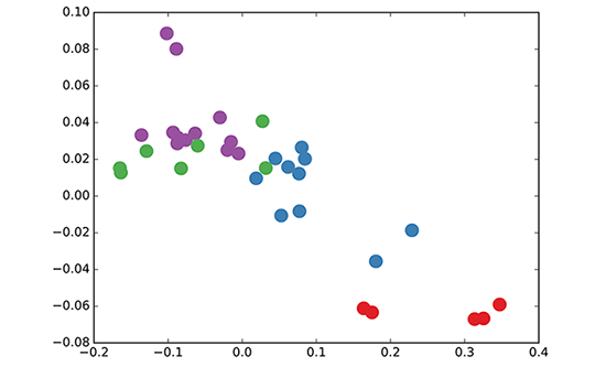
Next we simply label one node per class and use the semi-supervised learning algorithm for GCNs introduced in Kipf & Welling, ICLR 2017, and we start to train for a couple of iterations: The video above shows Semi-supervised classification with GCNs in this blog. And the model directly produces a 2-dimensional laten space which we can visualize.
Note that we just use random feature vectors (e.g., identity matrix we used here) and random weight matrices, only after a couple of iteration, the model used in Kipf & Welling is already able to achieve remarkable results. If we choose more serious initial node feature vectors, then the model can achieve state-of-the-art classification results on a various number of graph datasets.
Further Reading on GCN
Well, the GCN is developing rapidly, here are a few papers for further reading:
- Inductive Representation Learning on Large graph
- FastGCN: Fast Learning with Graph Convolutional Networks via Importance Sampling
- N-GCN: Multi-scale Graph Convolution for Semi-supervised Node Classification
Reference
- https://zhuanlan.zhihu.com/p/89503068
- https://towardsdatascience.com/how-to-do-deep-learning-on-graphs-with-graph-convolutional-networks-7d2250723780
- https://towardsdatascience.com/how-to-do-deep-learning-on-graphs-with-graph-convolutional-networks-62acf5b143d0
- https://tkipf.github.io/graph-convolutional-networks/
Li Wang
Research Fellow (Postdoctoral) on Computer Vision
My research focuses on image/video/geometry based neural style transfer.