Normalization_in_DL

Li Wang

Last updated on Jan 13, 2020 9 min read Computer Vision, DL

Batch Normalization (BN)

Short Description

Batch Normalization is a basic method to initialize inputs to neural networks. In the early years, the neural network is sensitive to the hyperparameters, which makes it difficult to train and stabilize. To address this problem, Loffe et al. proposed a novel normalization method to accelerate the neural network trianing process.

Training Problems

1. Slow learning speed. The $W$ weights and $b$ bias (parameters) in each layer are updated along with each SGD iterative optimization (back propagation), which makes the distribution of inputs to the next layer changes all the time. Thus the learning speed becomes slow as each layer has to adapt to input changes.

2. Slow convergence speed. For saturating nonlinearities like Sigmoid and Tanh, more and more inputs to activation functions may lay in the saturation regions along with the $W$ and $b$ increase. This further causes the gradient becomes close to 0 and weights update in a slow rate.

These problems are described as Internal Covariate Shift in Loffe et al. 2015.

Solutions to Internal Covariate Shift

1. Whitening (machine learning). Whitening aims to linearly transform the inputs to zero mean and unit variances, which decorrelates the inputs. There are normally two whitening methods: PCA and ZCA, where PCA whitening transforms inputs to zero mean and unit variance, and ZCA whitening transforms inputs to zero mean and same variance as original inputs.

2. Batch Normalization. Motivation: 1. whitening costs too much computation if it is put before each layer; 2. the distribution of transformed inputs does not have expressive power as original inputs.

Solutions:

simplify the linearly transformation by following equations: $$ \mu_j = \frac{1}{m}\Sigma_{i=1}^{m}{x_j^i}$$ $$\sigma^2_j = \frac{1}{m}\Sigma_{i=1}^{m}{(x_j^i - \mu_j)^2}$$ $$x_j^{i'} = \frac{x_j^i - \mu_j}{\sqrt{\sigma_j^2 + \varepsilon}}$$ where $j$ denotes the $j$th layer, $\mu_j$ and $\sigma_j^2$ denote the mean and variance of inputs $x_j$. $x_j^{i'}$ denotes the transformation output which has zero mean and unit variance, $m$ denotes the sample number in $x_i$ and $\varepsilon$ ($\varepsilon=10^{-8}$) prevents the zero in variance.
learn a linear transformation with parameter $\gamma$ and $\beta$ to restore original input distribution by following equation: $$x_j^{i"} = \gamma_j x_j^{i'} + \beta_j$$
where the transformed output will have the same distribution of original inputs when $\gamma_j^2$ and $\beta_i$ equal to $\sigma_j^2$ and $\mu_j$.

Normalization in testing stage. Generally, there may be just one or a few examples to be predicted in testing stage, the mean and variance computed from such examples could be baised. To address this problem, the $\mu_{batch}$ and $\sigma^2_{batch}$ of each layer are stored to compute the mean and variance for testing stage. For example, $\mu_{test} = \frac{1}{n} \Sigma \mu_{batch}$ and $\sigma^2_{batch}=\frac{m}{m-1} \frac{1}{n} \Sigma \sigma^2_{batch}$, then $BN(x_{test})=\gamma \frac{x_{test} - \mu_{test}}{\sqrt{\sigma^2_{test} + \varepsilon}} + \beta$.

Advantages of BN

Faster learning speed due to stable input distribution.
Saturating nonlinearities like Sigmoid and Tanh can still be used since gradients are prevented from disappearing.
Neural network is not sensitive to parameters, simplfy tuning process and stabilize the learning process.
BN partially works as regularization, increases generalization ability. The mean and variance of each mini -batch is different from each other, which may work as some noise input for the nerual network to learn. This has same function as Dropout shutdowns some neurons to produce some noise input to the neural networks.

Disadvantages of BN

NOT well for small mini-batch as the mean ans variance of small mini-batch differ great from other mini-batches which may introduce too much noise into the NN training.
NOT well for recurrent neural network as one hidden state may deal with a series of inputs, and each input has different mean and variance. To remember these mean and variance, it may need more BN to store them for each input.
NOT well for noise-sensitive applications such as generative models and deep reinforcement learning.

Rethink the resaon behind the effectiveness of BN

Why does the BN works so well in CNNs? This paper revisits the BN and proposes that the success of BN has little to do with reducing Internal Covariate Shift. Well, the ICS does exist in the deeper neural layers, but adding artifiical ICS after BN into a deep neural network, the added ICS does not affect the good performance of BN, which indicates that the performance of BN has little to do with ICS. Then what does the BN do to improve the training performance? The work mentioned above points out that BN smoothes the optimization landscape and makes the optimizer more easier to find the global minimic solution (c.f. Figure 4 in the paper). For more details, please refer to the paper.

Weight Normalization (WN)

Short description

Weight normalization is designed to address the disadvantages of BN which are that BN usually introduces too much noise when the mini-batch is small and the mean and variance of each mini-batch is correlated to inputs. It eliminates the correlations by normalizing weight parameters directly instead of mini-batch inputs.

Motivation and methodology

The core limitaion of BN is that the mean and variance is correlated to each mini-batch inputs, thus a better way to deal with that is design a normalization without the correlation. To achieve this, Salimans et al. proposed a Weight Normalization which is denoted as: $$w = \frac{g}{||v||} v$$ where $v$ denotes the parameter vector, $||v||$ is the Euclidean norm of $v$, and $g$ is scalar. This reparameterization has the effect of fixing the Euclidean norm of weight vector $w$, and we now have $||w||=g$ which is totally independent from parameter vector $v$. This operation is similar to divide inputs by standard deviation in batch normalization.

The mean of neurons still depends on $v$, thus the authors proposed a ‘mean-only batch normalization’ which only allows the inputs to subtract their mean but not divided by variance. Compared to variance divide, the mean subtraction seems to introduce less noise.

Layer Normalization

Short description

Layer normalization is inspired by batch normalization but designed to small mini-batch cases and extend such technique to recurrent neural networks.

Motivation and methodology

As mentioned in short description. To achieve the goal, Hinton et al. 2016 alter the sum statistic of inputs from batch dimension to feature dimension (multiple channels). For example, in a mini-batch (containing multiple input features), the computation can be described as following picture:

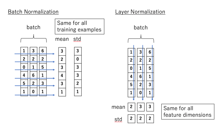
Fig 1. Layer Normalization Visualization

As can be seen, batch normalization computes the sum statistic of inputs across the batch dimension while layer normalization does across the feature dimension. The computation is almost the same in both normalization cases, but the mean and variance of layer normalization is independent of other examples in the same mini-batch. Experiments show that layer normalization works well in RNNs.

Instance Normalization (IN)

Short description

Instance normalization is like layer normalization mentioned above but it goes one step further that it computes mean and variance of each channel in each input feature. In this way, the statistic like mean and variance is independent to each channel. The IN is originally designed for neural style transfer which discovers that stylization network should be agnostic to the contrast of the style image. Thus it is usually specific to image.

Group Normalization (GN)

Short description

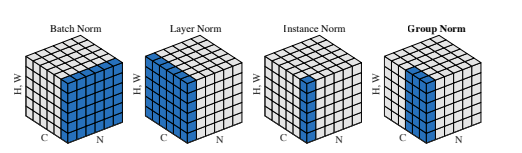
Group normalization computes the mean and variance across a group of channels in each training example, which makes it sound like a combination of layer normalization and instance normalization. For example, group normalization becomes layer normalization when all the channels are put into one single group, and becomes instance normalization when each channel is put into one single group. The picture below shows the visual comparisons of batch normalization, layer normalization, instance normalization and group normalization.

Motivation

Training small batch size with BN introduces noise into network which decreases the accuary. However, for larger models like object detection, segmentation and video, they have to require small batches considering the memory consumption. In addition, dependence bewteen channels widely exists but it is not extremely like all channels have dependences (layer normalization) or totally no dependence between channels (instance normalization). Based on this oberservation, He et al. 2018 proposed a group-wise normalization which divides the channels into groups and makes it flexiable for different applications.

Batch-Instance Normalization (BIN)

Short description

Batch-instance normalization is actually a interpolation of BN and IN, and lets the gradient descent to learn a parameter to interploates the weight of BN and IN. The equation below shows the defination of BIN:

$$BIN(x) = \gamma (\rho BN(x) + (1-\rho) IN(x)) + \beta$$ To some extend, this BIN inspires readers that models can learn to adaptively use different normalization methods using gradient descent. Would the network be capable of learning to use even wider range of normalization methods in one single model?

Motivation

Rethinking the instance normalization, Nam et al. 2019 regard instance normalization as an effective method to earse unnecessary style information from image and perserve useful styles for tasks like object classification, multi-domain learning and domain adaptation.

Switchable Normalization (SN)

Luo et al. 2018 investigated into whether different layers in a CNN needs different normalization methods. Thus they proposed a Switchable Normalization which learns parameters to switch normalizers between BN, LN and IN. As for results, their experiments suggest that (1) using distinct normalizations in different layer indeed improves both learning and generation of a CNN;(2) the normalization choices are more related to depth and batch size but less relevant to parameter initialization, learning rate decay and solver;(3) different tasks and datasets influence tha normalization choices. Additionally, the experiments in general also suggest that IN works well in early layers, LN works better in later layers while BN is preferred in middle layers.

Spectral Normalization

Spectral normalization (another form of weight normalization) is designed to improve the training of GANs by tuning the Lipschitz constant of the discriminator. The Lipschitz constant is a constant $L$ used in the following equation: $$||f(x) - f(y)|| \leqslant L ||x-y||$$

The Lipschitz constant is tuned by normalizing the weight matrices where is by their largest eigenvalue. And experiments show that spectral normalization stabilize the training by minimal tuning.

Conclusion

BN is a millstone research on training deep neural network which makes it much easier and more robust. However, the limitations like small batch size, noise-sensitie applications and distributed training still need to be fixed in further researches. And different applications/tasks may prefer different normalizations respect to accurancy. New dimensions of normalization still need to be discovered.

Reference:

Academic Normalization--Neual Network Optimization

Li Wang

Research Fellow on Computer Vision

My research focuses on image/video/geometry based neural style transfer.