Object_detection

This blog contains four parts:

1. Introduction: What is Object Detection? and general thoughts/ideas to deal with Object Detection;
2. Classic Deep Learning based Methods: multi-stage :RCNN and SPP Net , two-stage: Fast RCNN, Faster RCNN, Mask RCNN;
3. Classic One-Stage Methods: YOLOv1-v3, SSD, RetinaNet;
4. More Recent Anchor-Free Object Detection Methods (2018-2019);

1. Introduction

What is Object Detection? Given an image, object detection aims to find the categories of objects contained and their corresponding locations (presented as bounding-boxes) in the image. Thus Object Detection contains two tasks: classification and localization.

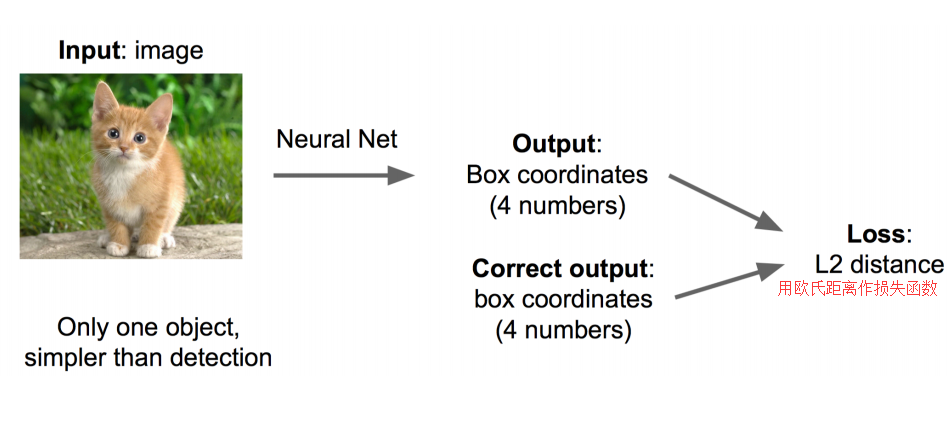
General thoughts/ideas to detect objects. The classification has been done by CNNs like AlexNet, VGG and ResNet. Then only localization still needs to be done. There are two intuitive ways: 1. Regression: the location of an object is presented by a vector $(x,y,w,h)$ which are the centre coordinates and width/height of an object bounding-box in the given image. For example, given an image, it only contains one object—cat. To locate the bounding-box, we apply a CNN to predict the vector $(x_p,y_p,w_p,h_p)$ and learn to regress the predicted vector to be close to groundtruth $(x_t,y_t,w_t,h_t)$ by calculating the L2 loss (see Fig 1.).

If the initial bounding-box is randomly chosen or there are many objects, then the entire regression will be much difficult and take lots of training time to correct the predicted vector to groundtruth. Sometime, it may not achieve a good convergence. However, if we select approximately initial box coordinates which probably contains the objects, then the regression of these boxes should be much easier and faster as these initial boxes already have closer coordinates to groundtruth than random ones. Thus, we could divide the problem into Box Selection and Regression, which are called Region Proposal Selection and Bounding-box Regression(please go post Basic_understanding_dl if you do not know Bounding-box regression) in Object Detection, respectively. Based on this, the early Object Detection methods contain multi-stage tasks like: Region Proposal Selection, Classification and Bounding-box Regression. In this blog, we only focus on the DL-based techniques, thus We do not review any pre-DL methods here.

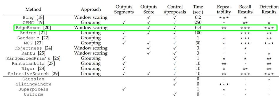
There are a few candidate Region Proposal Selection methods (shown in below), and some of them are able to select fewer proposals (nearly hundreds or thousands) and keep high recall.

2. Classic Deep Learning based Methods

Since using Region Proposal Selection can reduce bounding-box candidates from almost infinite to ~2k for one image with multiple objects, Ross et al. 2014 propose the first CNN-based Object Detection method, which uses CNN to extract features of images, classifies the categories and regress bounding-box based on the CNN features.

2.1 R-CNN (Region CNN)

The basic procedure of R-CNN model:

1. Use Selective Search to select ~2k Region Proposals for one image.
2. Warp all the Region Proposals into a same size as the fully connection layers in their backbone neural network (i.e., AlexNet) has image size limitation. For example, the FC layers only take 21x21xC feature vector as input, then all the input image size has to be 227x227 if all the Conv + BN + relu layers of a pre-trained AlexNet are preserved.
3. Feed the Region Proposals into the pre-trained AlexNet at each proposal per time rate, and extract the CNN features from FC7 layer for further classification (i.e., SVM).
4. The extracted CNN features will also be used for Bounding-box Regression.

Based on the procedure above, there are twice fine-tuning:

1. Fine-tune the pre-trained CNN for classification. For example, the pre-trained CNN (i.e., AlexNet) may have 1000 categories, but we may only need it to classify ~20 categories, thus we need to fine-tune the neural network.
2. Fine-tune the pre-trained CNN for bounding-box regression. For example, we add a regression head behind the FC7 layer, and we need to fine-tune the network for bounding-box regression task.

2.1.1 Some common tricks used

1. Non-Maximum Suppression

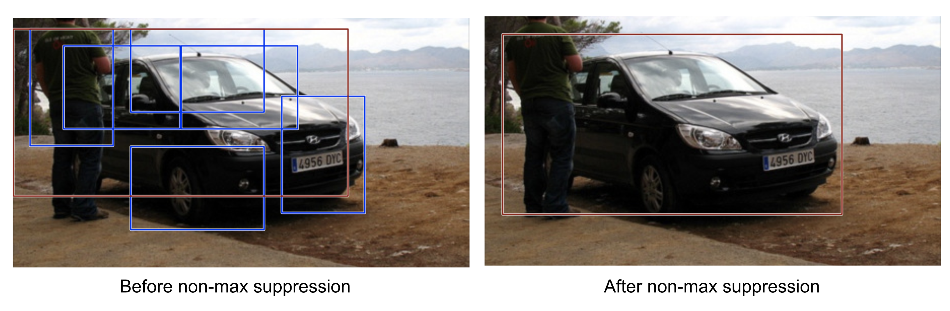
Commonly, sometimes the RCNN model outputs multiple bounding-boxes to localize the same object in the given image. To choose the best matching one, we use non-maximum suppression technique to avoid repeated detection of the same instance. For example, we have a set $B$ of candidate boxes, and a set $S$ of corresponding scores, then we choose the best box by following steps: 1. sort all the boxes with the scores, and remove the box $M$ with highest score from $B$, and add to set $D$; 2. check any box $b_i$ left in $B$, if the IoU of $b_i$ and $M$, remove $b_i$ from $B$; 3. repeat 1-2 until $B$ is empty. The box in $D$ is what we want.

2. Hard Negative Mining

Bounding-box containing no objects (i.e., cat or dog) are considered as negative samples. However, not all of them are equally hard to be identified. For example, some samples purely holding background are “easily negative” as they are easily distinguished. However, some negative samples may hold other textures or part of objects which makes it more difficult to identify. These samples are likely “Hard Negative”.

These “Hard Negative” are difficult to be correctly classified. What we can do about it is to find explicitly those false positive samples during training loops and add them into the training data in order to improve the classifier.

2.1.2 Problems of RCNN

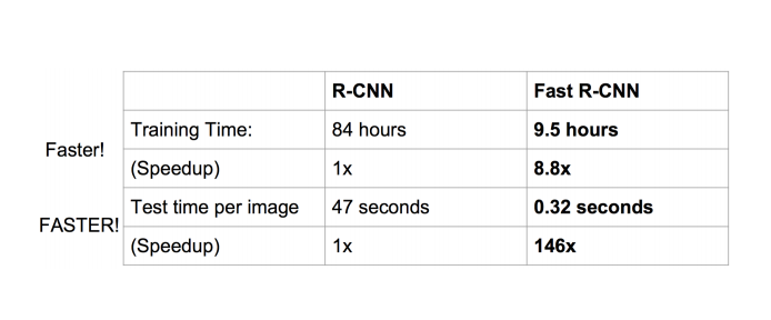
RCNN extracts CNN features for each region proposal by feeding each of them into CNN once at a time, and the proposals selected by Selective Search are approximately 2k for each image, thus this process consumes much time. Adding pre-processing Selective Search, RCNN needs ~47 second per image.

2.2 SPP Net (Spatial Pyramid Pooling Network)

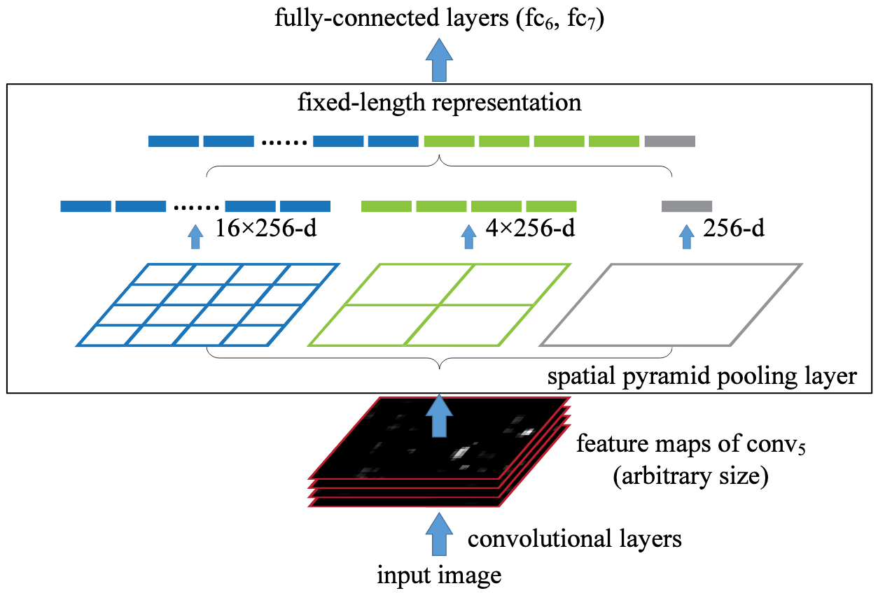
To speedup RCNN, SPPNet focuses on how to fix the problem that each proposal is fed into the CNN once a time. The reason behind the problem is the fully connected layers need fixed feature size (i.e., 1 x 21 x 256 in He et al.,2014) for further classification and regression. Thus SPPNet comes up with an idea that an additional pooling layer called spatial pyramid pooling is inserted right after the last Conv layer and before the Fc layers. The operation of this pooling first projects the region proposals to the Conv features, then divides each feature map (i.e., 60 x 40 x 256 filters) from the last Conv layer into 3 patch scales (i.e., 1,4 and 16 patches, see Fig 4. For example, the patch size is: 60x40 for 1 patch, 30x20 for 4 patches and 15x10 for 16 patches, next operates max pooling on each scaled patch to obtain a 1 x 21(1+4+16) for each feature map, thus we get 1x21x256 fiexd vector for Fc layers.

By proposing spatial pyramid pooling layer, SPPNet is able to reuse the feature maps extracted from CNN by passing the image once through because all information that region proposals need is shared in these feature maps. The only thing we could do next is project the region proposals selected by Selective Search onto these feature maps (How to project Region Proposals to feature maps? Please go to basic_understanding post for ROI pooling.). This operation extremely saves time consumption compared to extract feature maps per proposal per forward (like RCNN does). The total speedup of SPPNet is about 100 times compared to RCNN.

2.3 Fast RCNN

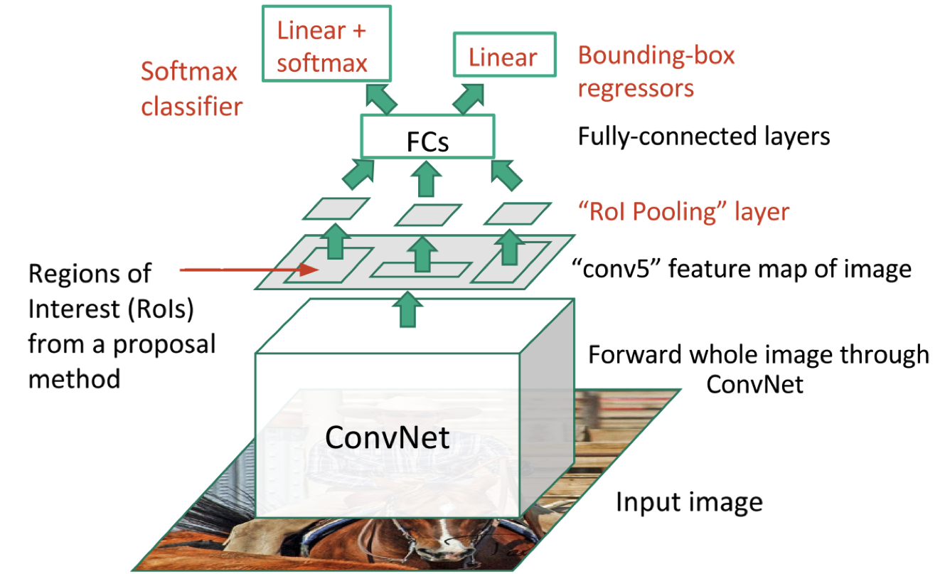
Fast RCNN attempts to overcome three notable drawbacks of RCNN:

1. Training a multi-stage pipeline: fine-tune a ConvNet based on Region Proposals; train SVM classifiers with Conv Features; train bounding-box regressors.
2. Training is expensive in space and time: 2.5 GPU-days for 5k images and hundreds of gigabytes of storage.
3. Speed is slow: ~47 second per image even on GPU.

Solutions:

1. Combine both classification (replace SVM with softmax) and bounding-box regression into one network with multi-task loss.
2. Introduce ROI pooling for: 1. reuse Conv feature maps of one image; 2. speedup both training and testing. Using VGG16 as backbone network, ROI (Region of Interest) pooling converts all different sizes of region proposals into 7x7x512 feature vector fed into Fc layers. Please go to post basic_understanding_dl for more details about ROI pooling.

Multi-task Loss for Classification and Bounding-box Regression

$——————————————————————————————–$

Symbol Explanation

$u$ Groundtruth class label, $u \in 0,1,…,K$; To simplify, all background class has $u=0$.

$v$ Groundtruth bounding-box regression target, $v=(v_x,v_y,v_w,v_h)$.

$p$ Descrete probability distribtion (per RoI), $p=(p_0,p_1,…,p_K)$ over $K+1$ categories. $p$ is computed by a softmax over the $K+1$ outputs of a fully connected layer.

$t^u$ Predicted bounding-box vector, $t^u=(t_x^u,t_y^u,t_w^u,t_h^u)$.

$——————————————————————————————–$

The multi-task loss on each RoI is defined as:

$$L(p,u,t^u,v) = L_{cls}(p,u) + \lambda[u \geqslant 1]L_{loc}(t^u,v)$$ where $L_{cls}(p,u)$=-log$p_u$ is a log loss for groundtruth class $u$. The Iverson bracket indicator function $[u \geqslant 1]$ is 1 when $u \geqslant 1$ (the predicted class is not background), and is 0 otherwise. The $L_{loc}$ term is using smooth L1 loss, which is denoted as: $$L_{loc}(t^u,v)=\sum_{i \in {x,y,w,h}}smooth_{L_1}(t_i^u-v_i)$$ and \begin{equation} smooth_{L_1}(x) = \begin{cases} 0.5x^2, \ |x| < 1 \newline |x|-0.5, \ otherwise \end{cases} \end{equation} $smooth_{L_1}(x)$ is a robust $L_1$ loss that is less sensitive to outliers than $L_2$ loss.

2.4 Faster RCNN

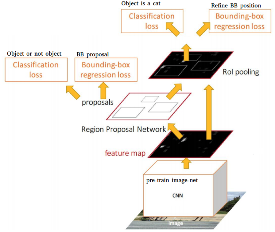
Faster RCNN focuses on solving the speed bottleneck of Region Proposal Selection as previous RCNN and Fast RCNN separately compute the region proposal by Selective Search on CPU which still consumes much time. To address this problem, a novel subnetwork called RPN (Region Proposal Network) is proposed to combine Region Proposal Selection into ConvNet along with Softmax classifiers and Bounding-box regressors.

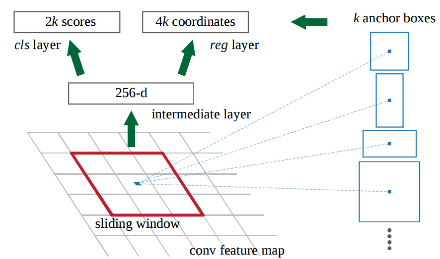
To adapt the multi-scale scheme of region proposals, the RPN introduces an anchor box. Specifically, RPN has a classifier and a regressor. The classifier is to predict the probability of a proposal holding an object, and the regressor is to correct the proposal coordinates. Anchor is the centre point of the sliding window. For any image, scale and aspect-ratio are two import factors, where scale is the image size and aspect-ratio is width/height. Ren et al., 2015 introduce 9 kinds of anchors, which are scales (1,2,3) and aspect-ratio(1:1,1:2,2:1). Then for the whole image, the number of anchors is $W \times H \times 9$ where $W$ and $H$ are width and height, respectively.

$——————————————————————————————-$

Symbol Explanation

$i$ the index of an anchor in a mini-batch.

$p_i$ the probability that the anchor $i$ being an object.

$p_i^{*}$ the groundtruth label $p_i^{*}$ is 1 if the anchor is positive, and is 0 if the anchor is negative.

$t_i$ a vector $(x,y,w,h)$ representing the coordinates of predicted bounding box.

$t_i^{*}$ that of the groundtruth box associated with a positive anchor.

$——————————————————————————————-$

The RPN also has a multi-task loss just like in Fast RCNN, which is defined as:

$$L({p_i},{t_i}) = \frac{1}{N_{cls}} \sum_i L_{cls}(p_i,p_i^{*}) + \lambda \frac{1}{N_{reg}} \sum_i p_i^{*} L_{reg}(t_i, t_i^{*})$$ where the classification $L_{cls}$ is log loss over two classes (object vs not object). The regression loss $L_{reg}(p_i, p_i^{*}) = smooth_{L1}(t_i - t_i^{*})$. The term $p_i^{*} L_{reg}(t_i, t_i^{*})$ means the regression loss is activated if $p_i^{*}=1$ and is disabled if $p_i^{*}=0$. These two loss term are normalized by $N_{cls}$ and $N_{reg}$ and weighted by a balancing parameter $\lambda$. In implementation, $N_{cls}$ is the number of images in a mini-batch (i.e., $N_{cls}=256$), and the $reg$ term is normalized by the number of anchor locations (i.e., $N_{reg} \sim 2,400$). By default, the $\lambda$ is set to 10.

Therefore, there are four loss functions in one neural network:

1. one is for classifying whether an anchor contains an object or not (anchor good or bad in RPN);
2. one is for proposal bounding box regression (anchor -> groundtruth proposal in RPN);
3. one is for classifying which category that the object belongs to (over all classes in main network);
4. one is for bounding box regression (proposal -> groundtruth bounding-box in main network);

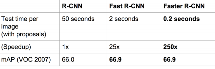
The total speedup comparison between RCNN, Fast RCNN and Faster RCNN is shown below:

2.5 Mask RCNN

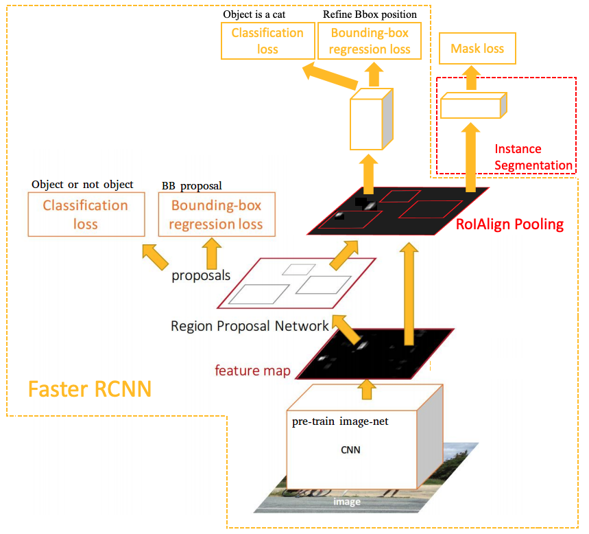
Mask RCNN has three branches: RPN for region proposal + (a pretrained CNN + Headers for classification and bounding-box regression) + Mask Network for pixel-level instance segmentation. Mask RCNN is developed on Faster RCNN and adds RoIAlign Pooling and instance segmentation to output object masks in a pixel-to-pixel manner. The RoIAlign is proposed to improve RoI for pixel-level segmentation as it requires much more fine-grained alignment than Bounding-boxes. The accurate computation of RoIAlign is described in RoIAlign Pooling for Object Detection in Basic_understanding_dl post.

Mask Loss

During the training, a multi-task loss on each sampled RoI is defined as : $L=L_{cls} + L_{bbox}+L_{mask}$. The $L_{cls}$ and $L_{bbox}$ are identical as those defined in Faster RCNN.

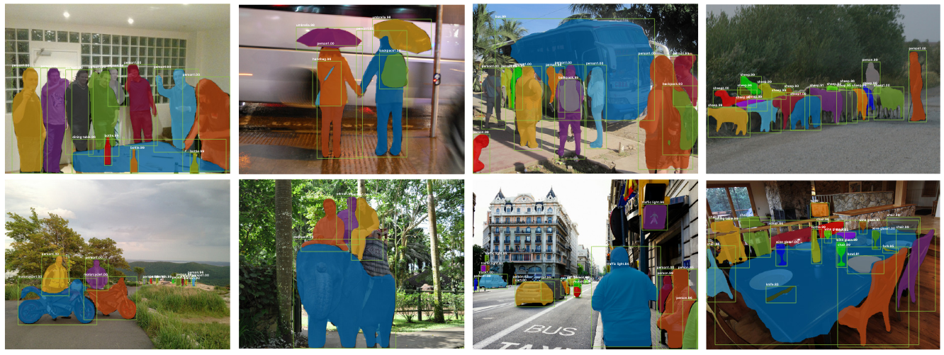
The mask branch has a $K\times m^2$ dimensional output for each RoI, which is $K$ binary masks of resolution $m \times m$, one for each the $K$ classes. Since the mask branch learns a mask for every class with a per-pixel sigmoid and a binary cross-entropy loss, there is no competition among classes for generating masks. Previous semantic segmentation methods (e.g., FCN for semantic segmentation) use a softmax and a multinomial cross-entropy loss, which causes classification competition among classes.

$L_{mask}$ is defined as the **average binary mask loss**, which **only includes $k$-th class** if the region is associated with the groundtruth class $k$: $$L_{mask} = -\frac{1}{m^2} \sum_{1 \leqslant i,j \leqslant m} (y_{ij}log\hat{y}_{ij}^k +(1-y_{ij})log(1-\hat{y}_{ij}^k))$$ where $y_{ij}$ is the label (0 or 1) for a cell $(i,j)$ in the groundtruth mask for the region of size $m \times m$, $\hat{y}_{ij}$ is the predicted value in the same cell in the predicted mask learned by the groundtruth class $k$.

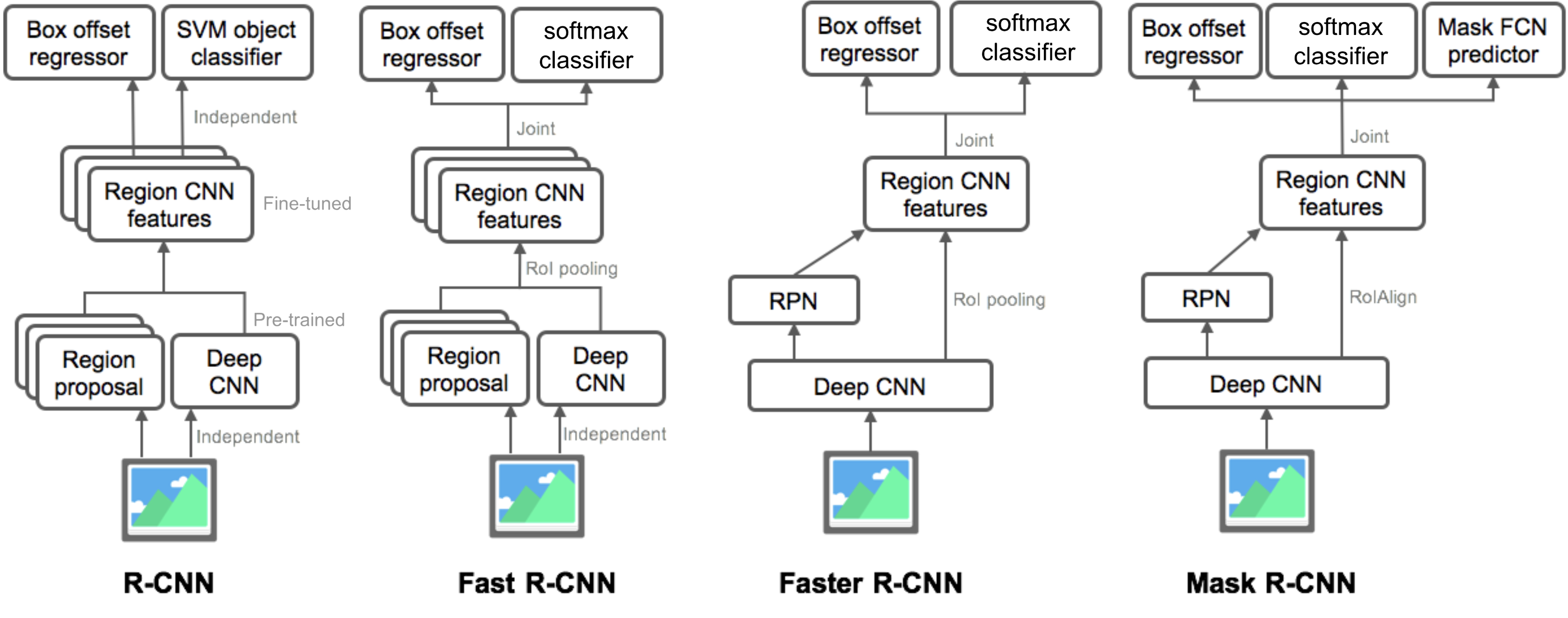
2.6 Summary for R-CNN based Object Detection Methods

3. Classic One-Stage Methods

3.1 YOLO (You Only Look Once)

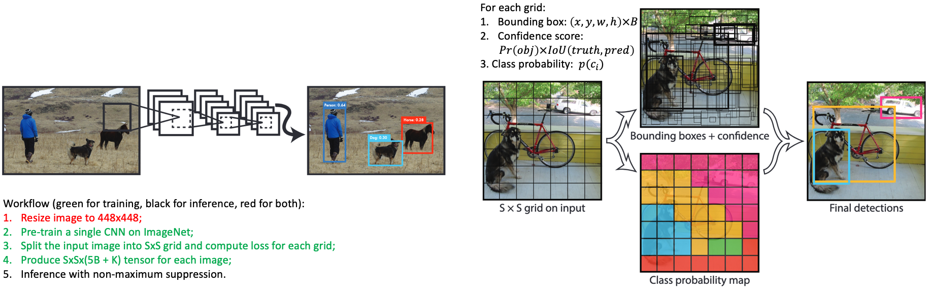
Introduction. YOLO is the first approach removing region proposal and learns an object detector in an end-to-end manner. Due to no region proposal, it frames object detection as a total regression problem which spatially separates bounding boxes and associated class probabilities. The proposed YOLO performs extremely fast (around 45 FPS), but less accuracy than main approaches like Faster RCNN.

3.1.1 Pipeline

1. Resize input image from 224x224 to 448x448;

2. Pre-train a single CNN (DarkNet similar to GoogLeNet: 24 conv layer + 2 fc) on ImageNet for classification.

3. Split the input image into $S \times S$ grid, for each cell in the grids:

   3.1. predict coordinates of B boxes, for each box coordinates: $(x,y,w,h)$ where $x$ and $y$ are the centre location of box, $w$ and $h$ are the width and height of box.

   3.2. predict a confidence score, $C = Pr(obj) \times IoU(trurh, pred)$ where $Pr(obj)$ denote whether the cell contains an object, $Pr(obj)=1$ if it contains an object, otherwise $Pr(obj)=0$. $IoU(truth, pred)$ is the interaction under union.

   3.3. predict a probability for every class, $p(c_i)$ where $i$ $\in$ {$1,2,…,K$} if a cell contains an object. During this stage, each cell only predicts one set of class probabilities regardless of the number of predicted bounding boxes $B$.

4. Output a $S \times S \times (5B + K)$ shape tensor after the last FC layer in total, then compute the loss.

5. In inference time, the network maybe outputs multiple candidate bounding boxes for one same object, then it uses non-maximum suppression to preserve the best match box.

3.1.2 Loss functions

$——————————————————————————————-$

Symbol Explanation

$\mathbb{1}_{ij}^{obj}$: an indicator function. It’s 1 when there is an object contained in the $j$-th predicted box of the $i$-th cell and $j$-th predicted box has the largest overlap region with the groundtruth box, otherwise it’s 0.

{$x_{ij}^p, y_{ij}^p, w_{ij}^p, h_{ij}^p$}: the centre coordinates and (width, height) of the predicted $j$-th bounding box in $i$-th cell.

{$x_{ij}^t, y_{ij}^t, w_{ij}^t, h_{ij}^t$}: the centre coordinates and (width, height) of the groundtruth $j$-th bounding box in $i$-th cell.

$C_{ij}^p$: the predicted confidence score for the $j$-th bounding box in $i$-th cell.

$C_{ij}^t$: the groundtruth confidence score for the $j$-th bounding box in $i$-th cell.

$p_i^{p}(c)$: the predicted class probability for $i$-th class category.

$p_i^{t}(c)$: the groundtruth class probability for $i$-th class category.

$\lambda_{coord}$: a weight parameter for coordinate loss. The default value is 5.

$\lambda_{noobj}$: a weight parameter for confidence score loss. The default value is 5.

$——————————————————————————————-$

The loss functions basically consists of three parts: coordinates $(x,y,w,h)$, confidence score $C$ and class probabilities $p(c_i)$, $i \in$ {$1,…,K$}. The total loss is denoted as: $$\begin{eqnarray} L_{total} &=& L_{loc} + L_{cls} \\\
&=& \lambda_{coor} \sum_{i=0}^{S^2} \sum_{j=0}^{B} \mathbb{1}_{ij}^{obj} ((x_{ij}^p - x_{ij}^t)^2 + (y_{ij}^p - y_{ij}^t)^2 + (\sqrt{w_{ij}^p} - \sqrt{w_{ij}^t})^2 + (\sqrt{h_{ij}^p} - \sqrt{h_{ij}^t})^2) \\\
&+& \sum_{i=0}^{S^2} \sum_{ij}^{B} (\mathbb{1}_{ij}^{obj} + \lambda_{noobj} (1 - \mathbb{1}_{ij}^{obj})) (C_{ij}^p - C_{ij}^t)^2 \\\
&+& \sum_{i=0}^{S^2} \mathbb{1}_{ij}^{obj} \sum_{c\in classes} (p_i^p(c) - p_i^t(c))^2 \end{eqnarray}$$

3.1.3 Differences ( or insights)

1. remove region proposal and complete the object detection task in an end-to-end manner.
2. the first approach achieves real-time speed.
3. the coordinate loss uses $(x,y,w,h)$ to represent bounding box, which is different from R-CNN based methods. This is because YOLO does not pre-define bounding boxes (i.e., region proposals or anchor boxes), thus YOLO can not use offset of coordinates to compute the loss or train the neural network.

3.1.4 Limitations

1. Less accurate prediction for irregular shapes of object due to a limited box candidates.
2. Less accurate prediction for small objects.

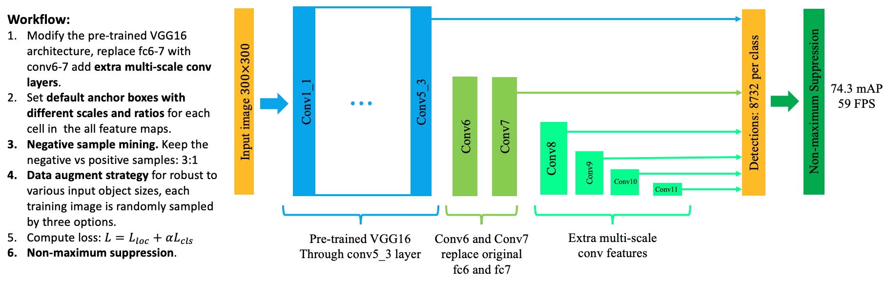
3.2 SSD (single shot multibox detector)

Introduction. SSD is one of early approaches attempts to detect multi-scale objects based on pyramid conv feature maps. It adopts the pre-defined anchor box idea but applies it on multiple scales of conv feature maps, which achieves real-time application via removing region proposal and high detection accuracy (even higher than Faster RCNN) via multi-scale object detection as well, e.g., it is capable of detecting both large objects and small objects in one image which increases the mAP.

3.2.1 Pipeline

1. Modify pre-trained VGG16 with replaced conv6-7 layers and extra multi-scale conv features. To detect multiple scales of input objects, a few (4 in this case) extra sizes of conv features are added into base model (see light green color in Fig14).
2. Several default anchor boxes with various scale and ratio (width/height) are introduced for each cell in all feature maps. For each of $m$ level conv feature maps, we compute the scale $s_k$, aspect ratio $a_r$, width $w_k^a$, height $h_k^a$ and centre location ($x_k^a, y_k^a$) of default boxes as:

• scale: $$s_k = s_{min} + \frac{s_{max} -s_{min}}{m-1}(k-1), k \in [1,m], s_{min}=0.2, s_{max}=0.9$$
• aspect ratio: $a_r \in$ {1,2,3,$\frac{1}{2}, \frac{1}{3}$}, additional ratio $s_k^{'}=\sqrt{s_k s_{k+1}}$, 6 default boxes in total.
• width: $w_k^a=s_k \sqrt{a_r}$
• height: $h_k^a= s_k / \sqrt{a_r}$
• centre location ($x_k^a, y_k^a$):$(\frac{i+0.5}{|f_k|}, \frac{j+0.5}{|f_k|})$ where $|f_k|$ is the size of the $k$-th square feture map, $i,j \in [0, |f_k|]$ .

where $s_{min}$ is 0.2 and $s_{max}$ is 0.9, which means the lowest layer has a scale of 0.2 and the highest layer has a scale of 0.9. Therefore, for each input object, there are $\sum_{i=0}^m C_i \times 6$ anchor boxes where $C_i$ is the channel of $i$-th level feature maps. And for all the multiple level feature maps, there are $\sum_{i=0}^{m} C_i H_i W_i \times 6$ anchor boxes in total where $H_i$ and $W_i$ are the height and width of $i$-th level feature maps.

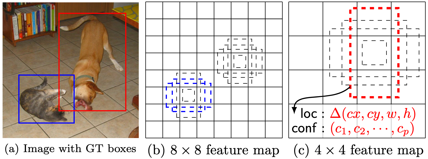
Advantage of pre-defined anchor boxes in SSD (matching strategy). During training, we first match each groundtruth box to the default box with highest jaccard overlap, then match default boxes to any groundtruth boxes with jaccard overlap higher than a threshold (0.5). This enables SSD to predict multiple high scores for multiple overlapping default boxes rather than requiring it to pick only the one with maximum overlap. Thus the network learns match suitable scale of default boxes to groundtruth box. For example, in Fig 15, the network learns from training that anchor boxes of dog on higher layer $4 \times 4$ are matched to groundtruth as the scale of anchor boxes on one $8 \times 8$ feature map are too small to cover the large size of dog.

3. Hard negative mining. During training, the number of input objects (or labeled anchor boxes) is quite smaller compared to the total number of default anchor boxes, thus most of them are negative samples. This introduces a significant imbalance between negative and positive training examples. The authors of SSD narrow down negative samples by choosing default boxes of top confidence loss, which makes sure the ratio between negative and positive samples at most 3:1.

4. Data augmentation (this contributes most improvement). To make the detector more robust to various input object sizes, SSD introduces a data augmentation which choose training samples by three following options:

• use the original input image
• sample a patch of original input image, whose IoU with its corresponding groundtruth box is 0.1,0.3,0.5,0.7 or 0.9.
• randomly sample a patch of the original input image.

The size of sampled patch is [0.1,1] of the original input image and its aspect ratio is between $\frac{1}{2}$ and 2. The overlapped region of the groundtruth box is kept if the centre of it is in the sampled patch. After the sampling step above, all the sampled patches are resized to fixed size and is horizontally flipped with probabilitiy of 0.5.

5. Compute the loss functions.
6. Non-maximum suppression to find the best match predicted boxes.

3.2.2 Loss functions

The training objective is the weighted combination of a localization loss and a classification loss: $$L = \frac{1}{N}(L_{loc} + \alpha L_{cls})$$ where $N$ is the number of matched boxes and $\alpha$ is picked by cross validation.

The localization loss is the smooth L1 between the predict offset of default boxes and those of matched groundtruth boxes, which is as same as the bounding box regression in RCNN:

$$L_{loc} = \sum_{i=0}^N \sum_{j\in(cx,cy,w,h)} \mathbb{1}_{ij}^k smooth_{L1}(\Delta t_{j}^i - \Delta p_{j}^i)$$ $$\Delta t_{cx}^i = (g_{cx}^i - p_{cx}^i) / p_w^i, \Delta t_{cy}^i = (g_{cy}^i - p_{cy}^i) / p_h^i,$$ $$\Delta t_{w}^i = log(\frac{g_{w}^i}{p_{w}^i}), \Delta t_{h}^i = log(\frac{g_{h}^i}{p_{h}^i}),$$ where $\Delta t_{j}^i$ is the offset of groundtruth boxes, and $\Delta p_{j}^i$ is the offset of predicted boxes. $\mathbb{1}_{ij}^k$ is an indicator for matching $i$-th default box to the $j$-th ground truth box of category $k$.

The classification loss is the softmax loss over multiple classes confidences ($c$) using cross entropy loss: $$L_{cls} = - \sum_{i=0}^N \mathbb{1}_{ij}^k log(\hat{c}_i^k) - \sum_{j=0}^M log(\hat{c}_j^0), \hat{c}_i^k = softmax(c_i^k) $$ where $N$ and $M$ indicates the positive and negative samples, $c_{i}^k$ is the predicted class probability for $k$-th object class, and $c_i^0$ is the predicted negative probability for non-object class (or background class).

3.2.3 Differences (or insights)

1. Multi-scale object detection via extra multiple scales of conv feature maps and matching strategy between default anchor boxes and ground truth boxes.
2. Training tricks: hard negative mining and data augmentation which increases the mAP most.

3.2.4 Limitations

Some posts (e.g., this blog and this blog) point out that matching strategy may not help to improve the prediction accuracy for smaller object as it basically only depends on lower layers with high resolution feature maps. These lower layers contain less information for classification. (well, I have not done further experiments to prove this).

3.3 YOLOv2/YOLO9000

YOLOv2 is an improvement version of YOLOv1 with several fine-tuning tricks (including adding anchor boxes, multi-scale training etc. see next section), and YOLO9000 is built on top of YOLOv2 but with a joint training strategy of COCO detection dataset and 9000 classes from ImageNet. The enhanced YOLOv2 achieves higher detection accuracy (including bounding box prediction and classification) and even more faster speed (480x480,59FPS) than SSD.

3.3.1 Tricks in YOLOv2

Batch Normalization. YOLOv2 adds BN after each convolutional layer and it helps to fast convergence, and increases the mAP about 2.4%.

High Resolution Classifier. YOLOv1 fine-tunes a pre-trained model with 448x448 resolution image from detection dataset (e.g., COCO). However, the pre-trained model is trained with 224x224 resolution images, which means directly fine-tuning this pre-trained model with higher resolution will not extract features with powerful expression of images. To address this problem, YOLOv2 first trains the pre-trained model with 448x448 resolution images for classification task, then trains the model with high resolution images for detection task. The high resolution is multiple of 32 as its network has 32 stride.

Convolutional Anchor Boxes. Instead of using 2 fc layers to regress the location of bounding boxes, inspired by RPN with anchor boxes, YOLOv2 uses convolutional layers and anchor boxes to predict bounding boxes and confidence scores. Each anchor box has a predicted $K$ class probability, thus the spatial location of anchor boxes and classification is decoupled. By adding anchor boxes, the mAP of YOLOv2 decreases a bit but it increases recall from 81% to 88%.

Dimension Clusters. Unlike the sizes of anchor box in Faster RCNN are hand-made, YOLOv2 chooses sizes of anchor box better suit to groundtruth bounding boxes. To find more suitable sizes, YOLOv2 uses k-means to cluster groundtruth bounding boxes and choose the sizes of anchor boxes more close to the centroid of each cluster by the following distance metric: $$d(box, centroid) = 1 - IoU(box, centroid)$$ and the best number of centroid $k$ can be chosen by the elbow method.

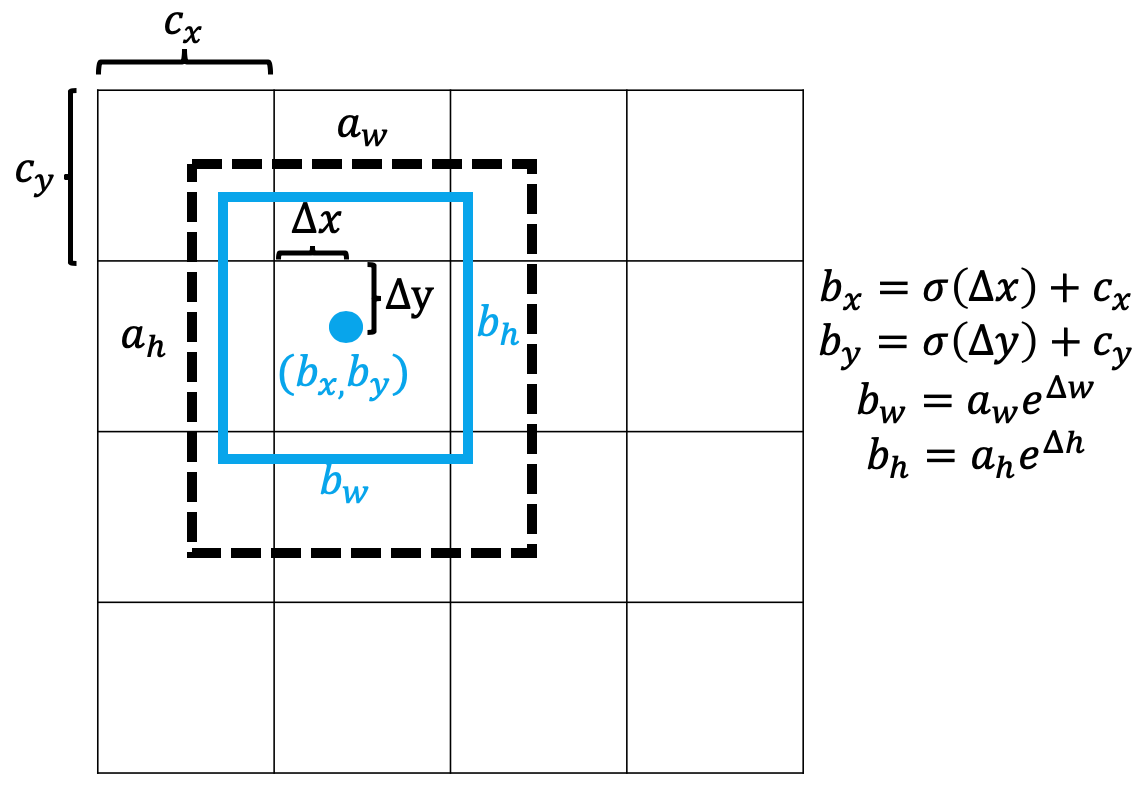
Direct location prediction. In Faster RCNN, the offset of an anchor box is predicted by the detector, and it is presented by ($\Delta x,\Delta y, \Delta w,\Delta h$). Then the predicted centre location of a bounding box is: $$x_p=x_a+(\Delta x \times w_a), y_p=y_a+(\Delta y \times h_a)$$ where $x_a$ and $y_a$ are centre location of an anchor box, $w_a$ and $h_a$ are the width and height. The centre location of a predict bounding box can be anywhere in a feature map, for example, if $\Delta x=1$, then the predicted $x_p$ will more a width distance horizontally from $x_a$. This is not good to locate the bounding boxes and could make training unstable. Therefore, YOLOv2 decides to predict the offset to the top-left corner ($c_x,c_y$) of a grid which the anchor box locates at. The scale of a grid is default 1. Then the location ($b_x,b_y,b_w,b_h$) of predicted bounding box is formulated as: $$b_x = (\sigma(\Delta x) \times 1) + c_x, b_y = (\sigma(\Delta y) \times 1) + c_y$$ $$b_w=a_w e^{\Delta w}, b_h=a_w e^{\Delta h}$$ where $\sigma(\cdot)=sigmoid(\cdot)$, $a_w$ and $a_h$ are width and height of an anchor box, and the width and height of the grid is set default 1. In this way, the movement of $b_x$ and $b_y$ is constrained in the grid as their maximum move distance is $\sigma(\cdot) \times 1 = 1$. Combining dimension clustering and direct location prediction increases mAP by 5%. The below figure illustrates the process:

Add fine-grained feature via passthrough layer. Inspired by ResNet, YOLOv2 also designs a passthrough layer to bring the fine-grained features from an earlier layer to the last output layer. This increases the mAP about 1%.

Multi-scale Training. To be robust to various input sizes, YOLOv2 inserts a new size of randomly sampled input images every 10 batches. The new sizes are multiple of 32 as its stride is 32.

Light-weighted base model. YOLOv2 use DarkNet-19 as base model which has 19 conv layers and 5 maxpooling layers. The key point is to add global avg pooling and 1x1 conv layers between 3x3 conv layers. This does not increases significant mAP but decreases the computation by about 33%.

3.3.2 YOLO9000: Joint Training of Detection and Classification

Since drawing bounding boxes in images for detection is much more expensive than tagging image for classification, the paper proposes a joint training strategy which combines small detection dataset and large classification dataset, and extand the detection from around 100 categories in YOLOv1 to 9000 categories. The name of YOLO9000 comes from the top 9000 classes of ImageNet. If one input image is from classification dataset, then the network only back propagates the classification loss during training.

The small detection dataset basically has the coarse labels (e.g., cat, person), while the large classification dataset may contain much more detailed labels (e.g., persian cat). Without mutual exclusiveness, this does not make sense to apply softmax to predict all over the classes. Thus YOLO9000 proposes a WordTree to combine the class labels into one hierarchical tree structure with reference to WordNet. For example, the root node of the tree is a physical object, then next level is coarse-grained labels like animal and artifact, then next level is more detailed labels like cat, dog, vehicle and equipment. Thus, physical object is the parant node of animal and artifact, and animal is the parent node of cat and dog. The labels on the same level should be classified by softmax as they are mutual exlusive.

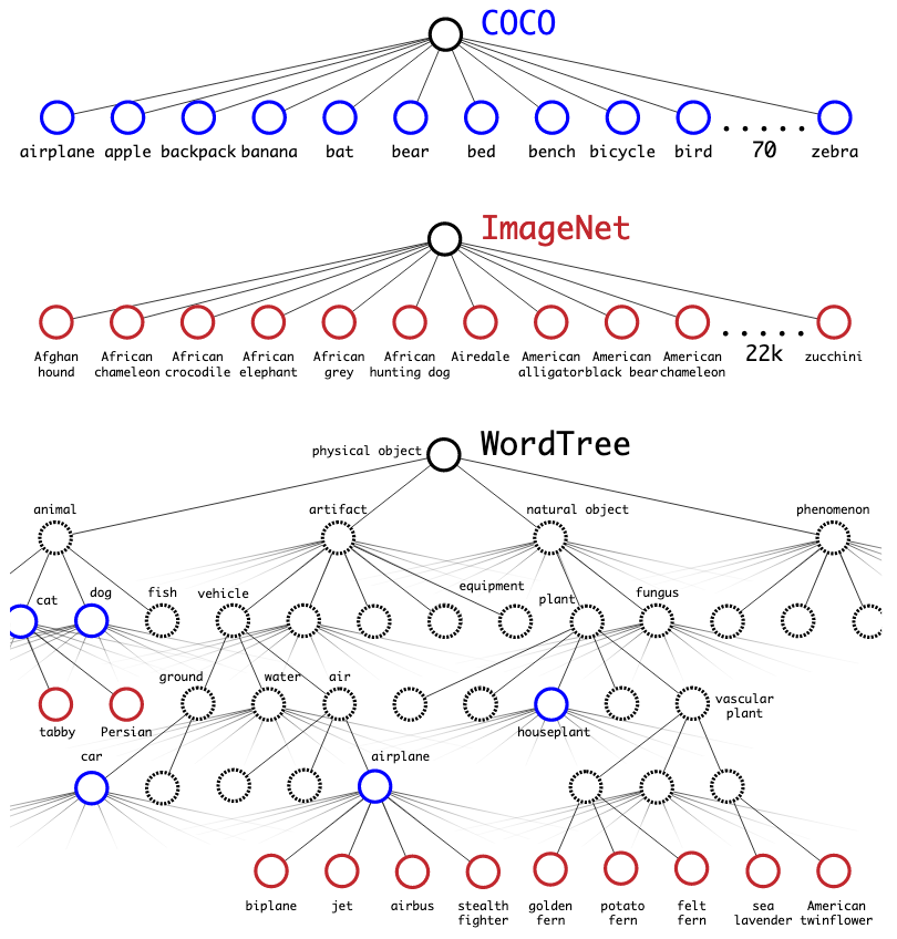
To predict the probability of a class node, we follow the path one node to the root, the searching stops when the probability is over a threshold. For example, the probability of a class label persian cat is: \begin{eqnarray} Pr(perisan \ cat \ | \ contain \ a \ physical \ object) &=& Pr(persian \ cat \ | \ cat) \\\
&\times& Pr(cat \ | \ animal) \\\
&\times& Pr(animal \ | \ physical \ object) \end{eqnarray} where $Pr(animal \ | \ physical \ object)$ is the confidence score, predicted separately from the bounding box detection.

3.3.3 Differences (or insights)

1. Dimension clustering and direct location prediction gives the most contribution of increasing mAP.
2. Word Tree is a creative thing in YOLO9000.

3.3.4 Limitations ( or unsolved problems)

During training, the significant imbalance number between positive anchor boxes containing objects and negative boxes containing background still hinders further improvement of detection accuracy.

Insight Questions for Object Detection

Why does the measurement of object detection only use mAP but no classification measurement? Honestly, I don’t know.

Why does improving the classification (binary classification: contains objects of interests or not) increase the detection accuracy? Well, I think that better classification will reduce negative samples (including easy and hard negative examples), then the network focuses on learning more positive samples to predict bounding boxes, which increases the mAP.

4. RetinaNet

RetinaNet is an one-stage object detector, which proposes two critical contributions: 1. focal loss for addressing class imbalance between foreground containing objects of interest and background containing no object; 2. FPN + ResNet as backbone network for detecting objects at different scales.

4.1 Focal Loss

The extreme class imbalance between training examples is one critical issue for object detection. To address the problem, a focal loss is designed to increase weights for hard yet easily misclassified examples (e.g., background with noisy texture or partial object) and down-weight easy classified examples (e.g., background obviously contains no objects and foreground obviously contains object of interests).

Starting with normal Cross Entropy loss for binary classification:

$$CE(p,y) = -ylog(p) - (1-y)log(1-p)$$ where $y \in$ {0,1} is a groundtruth binary label which indicates a bounding box contains an object or not. $p \in$ [0,1] is the predicted probability of a bounding box containing an object (aka confidence score).

For notational convenience, let $p_t$:

\begin{equation} p_t = \begin{cases} p, \ &if \ y=1 \newline (1-p), \ &otherwise, \end{cases} \end{equation}
then $$CE(p,y) \ = \ CE(p_t) \ = \ -log(p_t)$$

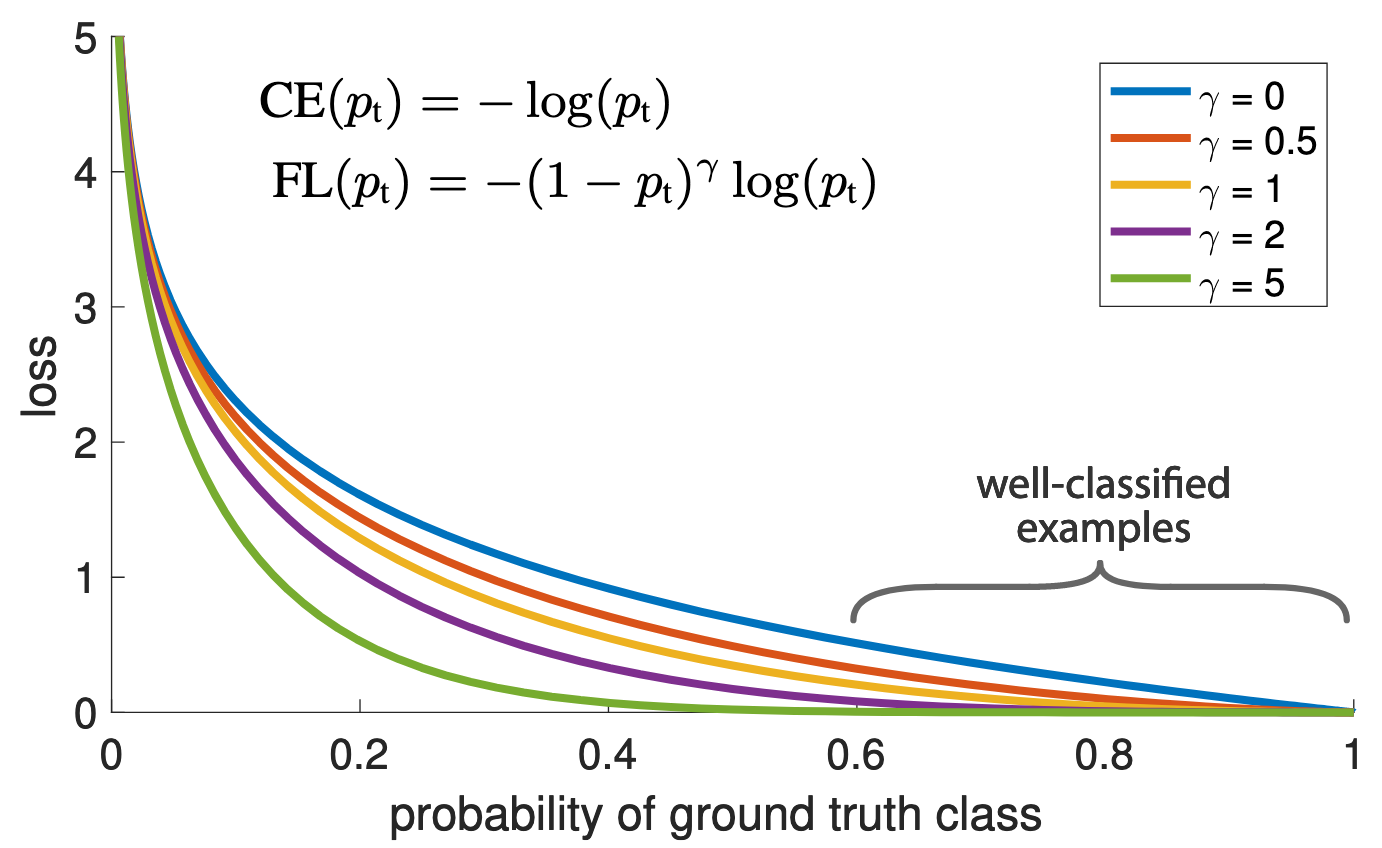
To down-weigh the $CE(p_t)$ when $p \gg 0.5$ (e.g., easily classified examples) and increase weight of loss when $p$ approaching 0 (e.g., hard classified examples), a focal loss is designed by adding a weight $(1-p_t)^\gamma$ into CE loss, which comes to the form:

$$FL(p_t) = -(1-p_t)^\gamma log(p_t)$$ here is the illustration of focal loss, as can be seen, easily classified examples with $p \gg 0.5$ is decreased and the loss of hard examples increases rapidly when $p$ is more closer to 0.

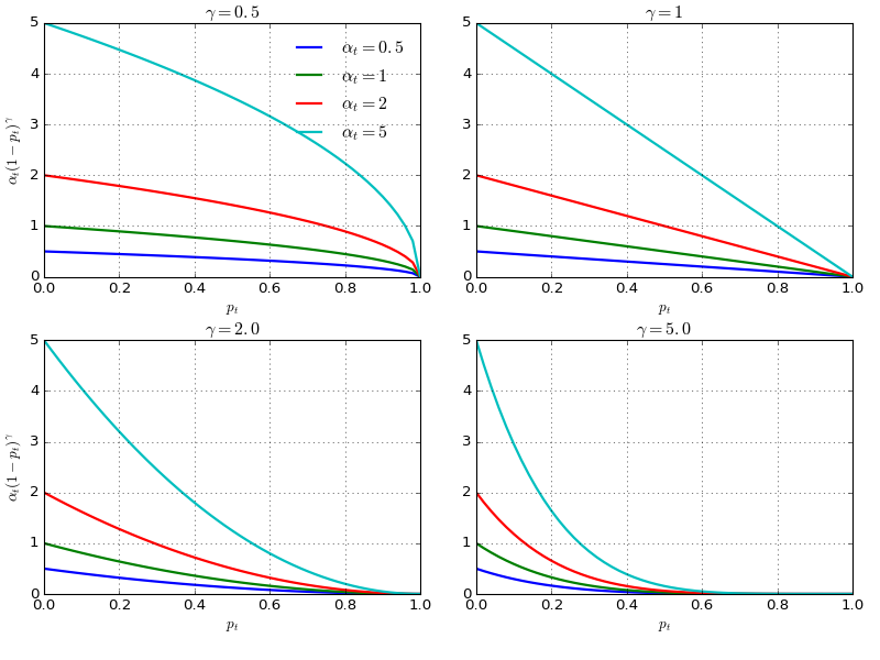
In practise, RetinaNet uses an $\alpha$-balanced variant of the focal loss: $$FL(p_t) = - \alpha (1-p_t)^\gamma log(p_t)$$ and there are experiments prove this form slightly improves accuracy over the non-$\alpha$-balanced form. In addition, implementing the loss layer with sigmoid operation for computing $p$ results in greater numerical stability.

To better illustrate the $\alpha$-balanced FL form, here are a few weighted Focal Loss with various combinations of $\alpha$ and $\gamma$:

4.2 FPN + ResNet as Backbone Network

Feature Pyramid Network (FPN) proposes that the hierarchic feature pyramids boost the detection accuracy. Thus, RetinaNet exploits this feature pyramid into their backbone network. Here is a brief introduction about the FPN.

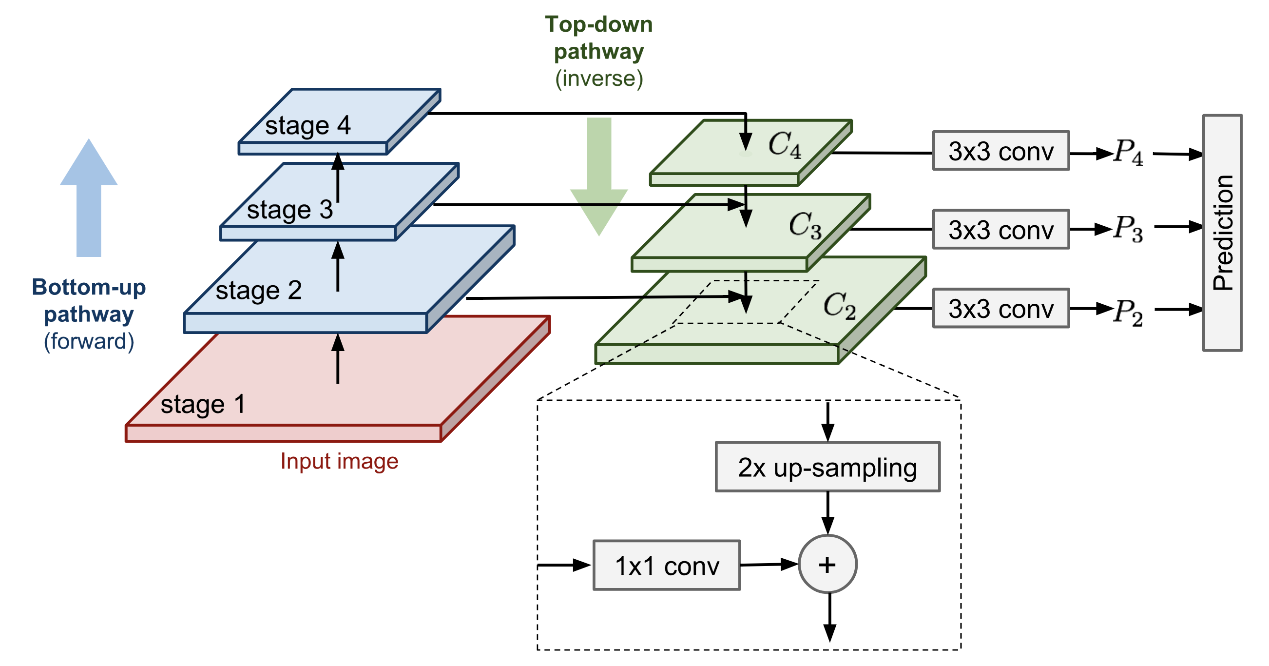
The key point of feature pyramid network is that multi-scale features in different stages are combined together via bottom-up and top-down pathways. For example, Fig 20, the basic pathways in FPN:

• bottom-up pathway: a forward pass via ResNet and features from different residual blocks (downscale by 2) form the scaled pyramid.
• top-down pathway: merges the strong semantic features from later coarse layer back to front fine layer by x2 upscale and 1x1 lateral connection and element-wise addition. The upscale operation is using nearest neighbour upsample in RetinaNet. While other upscale methods like deconv may also be suitable. The conv 1x1 lateral connection is to reduce the feature channel. The prediction happens after each top-down stage by a conv 3x3.

The improvement rank of these introduced components is as follows: 1x1 lateral connnect > detect object across multiple layers > top-down enrichment > pyramid representation (compared to only use single scale image like the finest layer).

4.3 Model Architecture

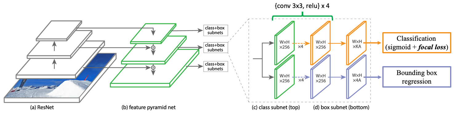
The basic model architecture of RetinaNet is built on top of ResNet by adding FPN and two subnets for classification and box regression. The ResNet has 5 residual blocks which are used to extract feature pyramid. Let $C_i$ denote the output of last conv layer of the $i$-th pyramid level (residual block) and $P_i$ denote the prediction based on $C_i$. As the downscale is 2 used between every two residual blocks, then $C_i$ is $2^i$ downscale lower than the original input image resolution.

RetinaNet uses prediction $P_s$ to $P_7$ for prediction, where:

• $P_3$ to $P_5$ are computed on features obtained from the element-wise addition of features after 1x1 conv $C_i$ (bottom-up pathway) and x2 upscaled $C_{i+1}$ (top-down pathway).
• $P_6$ is computed on features after 3x3 stride-2 conv on $C_5$.
• $P_7$ is computed on features after 3x3 stride-2 conv plus relu on $C_6$.

Prediction on higher level features leads to better detect large objects. In addition, all pyramid features are fixed to channel=256 as they share the same class subnet and box subnet.

The anchor boxes are also applied in RetinaNet, and they are set default to 3 scales {$2^0, 2^{\frac{1}{3}}, 2^{\frac{1}{2}}$} and 3 aspect ratios {$\frac{1}{2},1,2$}, thus 9 pre-defined anchor boxes in total. For each anchor box, the model predicts a classification probability for $K$ classes after passing through the class subnet (applying the proposed focal loss), and regresses the offset of the anchor box to the nearest groundtruth box via the box subnet.

4.3 Insights

1. Focal loss does a good job to address the imbalance between foreground containing objects of interests and background containing no object.
2. FPN+ResNet will be backbone for further one-stage object detectors.

YOLOv3

YOLOv3 proposes a series of incremental tricks for YOLOv2, and these tricks are inspired by recent researches:

1. logistic regression for objectiveness score (aka confidence score). Unlike using squared error for location loss in YOLOv1-2, YOLOv3 change this loss to a logistic loss to predict the offset of bounding boxes. The yolov3 paper tells that linear regression for predicting offset decreases in mAP.

2. independent logistic classifier instead of softmax for class prediction.

3. FPN works well in YOLOv3. YOLOv3 adopts the FPN to predict boxes at 3 different scales of features.

4. Features extracted from a new net called DarkNet-53. DarkNet-53 adopts the shortcut connections (residual blocks) from ResNet, and it performs similar to ResNet-152 but 2x faster.

Well, the authors of YOLO series tried focal loss, but it dropped mAP about 2 points. It maybe has something with no subnets for class and box prediction in YOLOv3, or the parameters $\lambda_{coord}$ and $\lambda_{noobj}$ in YOLO have done the job to balance the loss. Not sure yet.

Overall, YOLOv3 is still a good real-time object detector, it performs less accruacy than RetinaNet-101 (ResNet-101-FPN) but around 3.5~4.0x faster.

TO BE CONTINUED…

Reference

1. https://blog.csdn.net/v_JULY_v/article/details/80170182
2. https://lilianweng.github.io/lil-log/2017/12/31/object-recognition-for-dummies-part-3.html
3. https://medium.com/egen/region-proposal-network-rpn-backbone-of-faster-r-cnn-4a744a38d7f9
4. https://towardsdatascience.com/deep-learning-for-object-detection-a-comprehensive-review-
5. https://zhuanlan.zhihu.com/p/37998710
6. https://blog.csdn.net/heiheiya/article/details/81169758
7. https://lilianweng.github.io/lil-log/2018/12/27/object-detection-part-4.html
8. https://zhuanlan.zhihu.com/p/35325884