Specific_math

This post is an archive for some specific and easy forgotten mathematic knowledge like linear algebra and optimization behind ML/DL.

1. Linear Algebra

1.1 Rank of a matrix

Given $n$ number of math functions with $m$ variables and it is written as following:

\begin{eqnarray} &a_{11} x_1 + a_{12} x_2 + &a_{13} x_3 + &\cdot \cdot \cdot + a_{1m} x_{m} &= b_1 \\\
&a_{21} x_1 + a_{22} x_2 + &a_{23} x_3 + &\cdot \cdot \cdot + a_{2m} x_{m} &= b_2 \\\
&a_{31} x_1 + a_{32} x_2 + &a_{33} x_3 + &\cdot \cdot \cdot + a_{3m} x_{m} &= b_3 \\\
&\cdot \cdot \cdot &\cdot \cdot \cdot &\cdot \cdot \cdot &\cdot \cdot \cdot \\\
&a_{n1} x_1 + a_{n2} x_2 + &a_{n3} x_3 + &\cdot \cdot \cdot + a_{nm} x_{m} &= b_n \\\
\end{eqnarray}

If we extract all the coefficient from the math functions above, and name each row of coefficient as $\alpha_i$ where $i=(1,2,…,n)$, then we have a column of vectors ($\alpha_1, \alpha_2, …, \alpha_n$) and each of them is as following:

\begin{eqnarray} &(a_{11}, a_{12}, \cdot \cdot \cdot, a_{1m}) &= \alpha_1 \\\
&(a_{21}, a_{22}, \cdot \cdot \cdot, a_{2m}) &= \alpha_2 \\\
&\cdot\cdot\cdot \\\
&(a_{n1}, a_{n2}, \cdot \cdot \cdot, a_{nm}) &= \alpha_n \\\
\end{eqnarray}

Now we explain a noun called linear independent set consisting of $\alpha_i$. If each coefficient $k_i \in \mathbb{R}$ where $i=(1,2,…,s)$ have to be 0 like $k_1 = k_2 = \cdot \cdot \cdot = k_s = 0$ in order to make the following equation equal 0: $$k_1 \alpha_1 + k_2 \alpha_2 + \cdot \cdot \cdot + k_s \alpha_s = 0$$ then we say $(\alpha_1,\alpha_2,…,\alpha_s)$ is a linear independent set.

For a matrix, the Rank is the maximum number of $\alpha$ to be a linear independent set. In other words, Rank is the number of $\alpha$ in the maximal linear independent set.

For example, only if $k_1$ and $k_2$ have to be 0 to make sure $k_1 \alpha_1 + k_2 \alpha_2=0$, then we say $(\alpha_1, \alpha_2)$ is a linear independent set, and the number of this linear independent set is 2. Next, only if $k_1=k_2=k_3=0$ makes sure $k_1 \alpha_1 + k_2 \alpha_2 + k_3 \alpha_3=0$, then we say $(\alpha_1, \alpha_2, \alpha_3)$ is a linear independent set, and the number is 3. Continue, we firstly find that NOT all of $k_1$,$k_2$,…,$k_s$ and $k_{s+1}$ have to be 0 and it still makes $k_1 \alpha_1 + k_2 \alpha_2 + k_3 \alpha_3 + \cdot \cdot \cdot + k_s \alpha_s=0$ happen, then we say $(\alpha_1, \alpha_2, \alpha_3,…,\alpha_{s+1})$ is not a linear independent set. And we call $(\alpha_1, \alpha_2, \alpha_3,…,\alpha_{s})$ as the maximal linear independent set, and the number is $s$. If each $\alpha_i$ contains one row of coefficient in a series of equations, then the Rank of the matrix composed by all the coefficient is $s$.

1.2 Inverse of a matrix

If a matrix $A$ has $n$ rows and $n$ columns, which is named $A_{n \times n}$, and rank of $A_{n \times n}$ is equal to $n$, then the matrix has an inverse matrix. The definition of inverse of a matrix is, there is a matrix $B_{n \times n}$, which makes sure the following equation: $$AB=BA=I_n$$ where $I_n$ is the identity matrix (or unit matrix), of size $n \times n$ , with ones on the main diagonal and zeros elsewhere.

1.3 Positive Definite and Positive Semi-Definite Matrix

Definition of Positive Definite Matrix: Given a $n \times n$ matrix $A$, and $A$ is a real symmetric matrix (e.g., $A \in \mathbb{R}^{n \times n}$). If $\forall x \in \mathbb{R}^n$ made: $$x^T A x > 0$$, then matrix $A$ is a positive definite matrix.

Definition of Positive Semi-Definite Matrix: Given a $n \times n$ matrix $A$, and $A$ is a real symmetric matrix (e.g., $A \in \mathbb{R}^{n \times n}$). If $\forall x \in \mathbb{R}^n$ made: $$x^T A x \geq 0$$, then matrix $A$ is a positive semi-definite matrix.

2. Convex Optimization

An optimization is a convex optimization problem only if the objective function is a convex function and the range of variables is a convex set/domain.

The advantage of a convex optimization is that perhaps there are many local mimic points (where the gradient is equal to 0) but all of them are the best minimal point, which makes it easier to find a solution to an optimization problem.

2.1 Convex Set/Domain

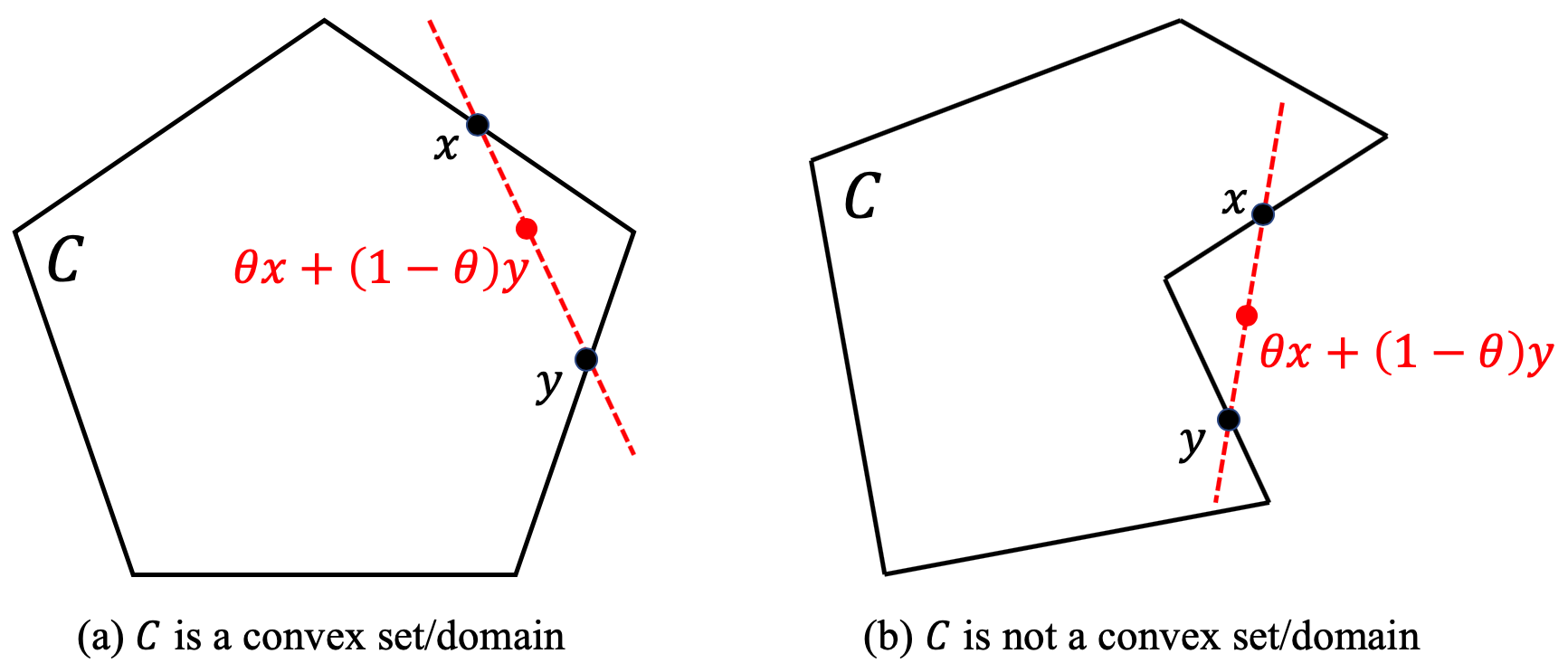
Then what is a convex set/domain? Definition: if there is a set of vectors called $C$ and the length of each vector is $n$, and for $\forall x,y \in C$, and one real number $\theta$ falls in the range of [0,1] (e.g., $0 \leq \theta \leq 1 $), the linear combination of $x$ and $y$: $$\theta x + (1-\theta) y \in C$$ then we call $C$ is a convex set/domain(see figure below).

A few sets we’ve already known are convex sets. For example, a real number set $\mathbb{R}$. It’s obvious that $\forall x,y \in \mathbb{R}$, and $\forall \theta \in \mathbb{R}$ and $0 \leq \theta \leq 1$: $$\theta x + (1-\theta) y \in \mathbb{R}$$ An affine subspace $\mathbb{R}^n$. Given a $n \times m$ matrix $A$ and a vector $b$ of length $m$, then an affine subspace is such a set consisting of the following elements:
$$\{x \in \mathbb{R}^n: Ax=b\}$$ Now we give the proof that an affine subspace is a convex set/domain. For $\forall x,y \in \mathbb{R}^n$, and $$Ax=b, \ Ay=b$$ then $\forall \theta$ and $0 \leq \theta \leq 1$: $$A(\theta x + (1-\theta)y) = A\theta x + A (1-\theta)y = \theta Ax + (1-\theta) Ay = \theta b + (1-\theta)b = b$$ thus, an affine subspace $\mathbb{R}^n$ is a convex set/domain.

A polyhedron space $\mathbb{R}^n$. Similar to an affine space, given a $n \times m$ matrix $A$ and a vector $b$ of length $m$, then a polyhedron space is such a set consisting of the following elements: $$\{x \in \mathbb{R}^n: Ax \leq b\}$$ Now we give the proof that a polyhedron space is a convex set/domain. For $\forall x,y \in \mathbb{R}^n$, and $$Ax \leq b, \ Ay \leq b$$ then $\forall \theta$ and $0 \leq \theta \leq 1$: $$A(\theta x + (1-\theta)y) = A\theta x + A (1-\theta)y = \theta Ax + (1-\theta) Ay \leq \theta b + (1-\theta)b = b$$ thus, a polyhedron space $\mathbb{R}^n$ is a convex set/domain.

The interaction of convex sets/domains is still a convex set. For an optimization problem, if all the variable sets/domains of constrains for the objective function are convex sets/domains, then the variable set satisfying all the constrains is still a convex set/domain.

2.2 Convex Function

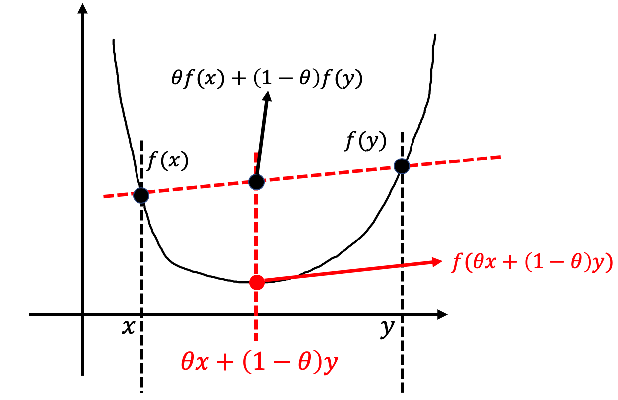
Then what is a convex function? Definition: in the domain of function, $\forall x,y$ and $0 \leq \theta \leq 1$, they always satisfy the following equation: $$f(\theta x + (1-\theta)y) \leq \theta f(x) + (1-\theta) f(y)$$ then function $f(x)$ is a convex function (see figure below).

How to determine whether a function is a convex function? For a function $f(x)$ with only one variable, if its second-derivative is equal or greater than 0, then this function is a convex function. For a function $f(x_1,x_2,…,x_n)$ with multiple variables, if the Hessian Matrix is a positive semi-definite matrix, then the function is a convex function.

For a function $f(x_1,x_2,…,x_n)$ contains multiple variables, its Hessian matrix is the partial derivative matrix:

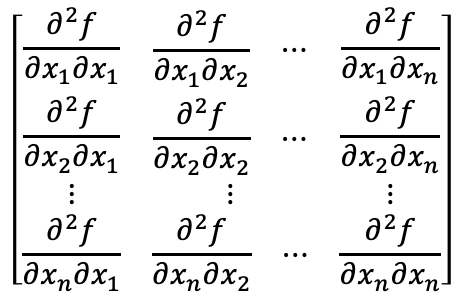
Since $\frac{\partial^2 f}{\partial x_i \partial x_j} = \frac{\partial^2 f}{\partial x_j \partial x_i}$ where $i,j \in $ {$1,2,…,n$}, then the Hessian matrix is symmetric matrix.

Next, if there is a point $M$=( $x_1^{'}$, $x_2^{'}$,…,$x_n^{'}$) satisfies $\lim_{x_i \to x_i^{'}} \frac{\partial f}{\partial x_i}=0$ where $i \in $ {$1,2,…,n$}, and if :

1. the Hessian Matrix is positive semi-definite or positive definite, then the value of $f(x_1^{'},x_2^{'},…,x_n^{'})$ is the global minimal value, and $M$ is the global mimic point.
2. the Hessian Matrix is negative semi-definite or negative definite, then the value of $f(x_1^{'},x_2^{'},…,x_n^{'})$ is the global maximal value, and $M$ is the global maximal point.
3. the Hessian Matrix is non-definite, then $M$ is a Saddle point of function $f(x_1,x_2,…,x_n)$.

2.3 Sub-level Set of a Convex Function

Given a convex function $f(x)$, and a real number $\alpha \in \mathbb{R}$, a sub-level set $S$ is defined as the set of variable $x$ that satisfies the values of $f(x)$ is equal or lower than $\alpha$:

$$\{ x \in S: f(x) \leq \alpha \}$$ According to the definition of a polyhedron set above, the sub-level set $S$ is a polyhedron set, which is also a convex set.

2.4 Convex Optimization

In general, a convex optimization is written as: $$\min_{x \in C} f(x)$$ where $f(x)$ is the objective convex function, $x$ is the variable and $C$ is a convex set/domain. To prove this optimization to be a convex optimization, we need to prove the objective function is a convex function and its variable set is a convex set. Another general format of a convex optimization is denoted as:

$$\min f(x)$$ and the constrains are: $$g_i(x) \leq 0, \ i=(1,2,…,m) \ and \ h_i(x)=0, \ i=(1,2,…,n)$$ according to the definitions above, if $g_i(x)$ is a convex function, then the variable set of $g_i(x)$ is a polyhedron set which is a convex set. $h_i(x)$ is an affine subspace, which is also a convex set. Then the interaction of these two convex sets is still a convex set.

The most important property of a convex optimization is that if we find a point that makes the gradient at this point to be 0, then this point is the global optimal solution. There are perhaps many points in variable set, but if we can find one of them, then we can stop.

2.5 The convex optimization used in Machine Learning

2.5.1 Linear regression

In machine learning, linear regression is a simple supervised learning algorithm. Given feature vectors $x_i$ and its corresponding groundtruth labels $y_i$ where $i =$ {$1,2,…,N$}, then the linear function can be written as: $$f(x)=w^T x + b$$ and the loss function is denoted as the mean square error between the value $f(x_i)$ and its corresponding label $y_i$: $$L = \frac{1}{2N} \sum_{i=0}^{N} (f(x_i) - y_i)^2$$ then we replace $f(x_i)$ with its function and get: $$L = \frac{1}{2N} \sum_{i=0}^{N} (w^T x_i + b - y_i)^2$$ if we assume that: $$[w, b] \rightarrow w, \ and \ [x, 1] \rightarrow x$$ then we get: $$L = \frac{1}{2N} \sum_{i=0}^{N} (w^T x_i - y_i)^2$$ and we get: $$L = \frac{1}{2N} \sum_{i=0}^{N} ((w^T x_i)^2 - 2 w^T x_i y_i + y_i^2)$$ and the partial derivative (I still do not know how to compute this partial derivative) is: $$\frac{\partial^2 L}{\partial w_i \partial w_i} = \frac{1}{N} \sum_{k=1}^N x_{k,i}x_{k,j}$$ then the Hessian Matrix is:

the Hessian Matrix can be written in matrix-format:

where $X$ is a column of vector $x_i$ ($i =$ {$1,2,…,N$}), we can prove that this Hessian Matrix is a positive semi-definite matrix. For example, $\forall x \in \mathbb{R}^N$ and $x \neq 0$: $$x^TX^TXx = (Xx)^T Xx \geq 0$$ thus the loss function of linear regression is a convex function without any constrains, we can find the global optimal solution by SGD or other methods.

2.5.2 Other ML algorithms

Similarly, we can use the same way to prove that the optimization problem of Logistic Regression $f(x)=\frac{1}{1+e^{-x}}$, Softmax $f(x) = \frac{e^{x_i}}{\sum_{j=0}^N e^{x_j}}$ and SVM is also a convex optimization. However, the optimization using Deep Neural Network is not a convex optimization thus people do not understand the mathematic behind it and regard it as a black-box.

Reference:

https://zhuanlan.zhihu.com/p/37108430